Introduction#
In the NetSim’s Internetworks library Wireless nodes connect to an Access Point (AP) while in NetSim’s LTE and 5G libraries, the mobile nodes (UEs) connect to base stations (eNBs, gNBs). There is no such association between the wireless stations and any fixed infrastructure in MANETs.
A Mobile Ad hoc Network (MANET) is an autonomous system of mobile nodes. In such networks, information transport services are built over a set of arbitrarily located nodes, which are possibly mobile. Every node behaves both like a mobile host and as a wireless router. There are many obvious applications for such networks including emergency communications, vehicular communications, military applications, etc.
Such networks have dynamic (sometimes rapidly changing), random, multi-hop topologies which are composed of relatively bandwidth-constrained wireless links. MANETs must therefore support efficient operation in mobile wireless environments by incorporating routing functionality into mobile nodes. Note that such multi-hop networks exploit spatial reuse; transmissions can occur simultaneously on links that are sufficiently separated in space.
In NetSim MANETs, data packets are sent between source-destination pairs by multi-hop relaying. The MANETs in NetSim may operate in isolation or may have bridge nodes to interface with other networks (wired networks, or even other MANETs). NetSim MANET library supports the following protocols.
- Layer 3 Unicast Routing
- Dynamic Source Routing (DSR)
- Adhoc On demand Distance Vector Routing (AODV)
- Optimized Link state Routing (OLSR)
- Zone Routing Protocol (ZRP)
- MAC / PHY (interfaced from NetSim Internetworks library)
- 802.11 a, b, g, n, ac. p and e
NetSim MANETs component can be interfaced with:
- NetSim Component 6 (IOT) module to run 802.15.4 in MAC/PHY
- NetSim Component 9 (VANETs) module to run IEEE 1609 WAVE in MAC/PHY
- NetSim TDMA Radio Networks (Add on) to run TDMA/DTDMA in MAC/PHY

The digital communication system employed, the transmit power used, and the radio propagation characteristics of the environment determine the “links” in the network.
Performance analysis of wireless ad hoc networks is a challenging task owing to the fact that such analysis must take into account the interactions between the wireless physical layer, radio propagation, multiple access, random topology, routing, and the characteristics of the application that generates the traffic carried by the network. Therefore, unlike wired and fixed topology networks, understanding and optimizing the performance of MANETs is a difficult undertaking, owing to the complex interaction between the various “layers” of the network.
Simulation GUI#
In the Main menu select →New Simulation→Mobile Adhoc networks as shown in below Figure

Fast Configuration#

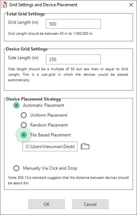
Fast Config window allows users to define device placement strategies and conveniently model large network scenarios especially in network such as MANET, TDMA Radio Networks, WSN and IoT. The parameters associated with the Fast Config Window is explained below:
Grid length: It is the area of simulation environment. Users can change the length of the grid in the range of 50-1000000m.
Side length: It specifies the area in the grid environment within which the devices will be placed. User can change the side length of the grid in the range of 50 - 1000000m.Side length should be multiple of 50. Side length should always be set to a value less than or equal to the Grid length.
Device Placement#
Automatic Placement#
- Uniform Placement: Devices will be placed uniformly with equal gap between the devices in area based on the side length. This requires users to specify the number of devices as square number. For Eg. 1, 4, 9, 16 etc.
- Random Placement: Devices will be placed randomly in the grid environment within the area based on side length.
- File Based Placement: In order to place devices in user defined locations file-basedplacement option can be used. The file has the following general format:
<DEVICE_NAME>,<DEVICE_TYPE>,<X_COORDINATE>,<Y_COORDINATE>
Where,
DEVICE_NAME – is any name that will be assigned to the device.
DEVICE_TYPE – is the unique Device Identifier specific to each type of device in NetSim.
Following table provides the DEVICE_TYPE’s of all possible devices for networks with support for Device Fast Configuration:
| NETWORK | DEVICE_TYPE |
|---|---|
| Manets | |
| 1. WIRELESSNODE | |
| 2. BRIDGE_WIREDNODE | |
| 3. BRIDGE_WIRELESSNODE | |
| 4. WIREDNODE | |
| 5. ROUTER | |
| 6.L2_SWITCH | |
| WSN | 1.Sensors |
| 2 .SinkNode | |
| IOT | 1 IOT_Sensors |
| 2 LOWPAN_Gateway | |
| 3.WIREDNODE | |
| 4. IOT_ROUTER | |
| 5. ACCESSPOINT | |
| 6. L2_SWITCH |
X_COORDINATE – the value of X coordinate of the device
Y_COORDINATE – the value of Y coordinate of the device
Eg: MANET_File_based_Placement.txt
Wireless_Node,WIRELESSNODE,100,150
Wireless_Node,WIRELESSNODE,150,100
Wireless_Node,WIRELESSNODE,100,100
Wireless_Node,WIRELESSNODE,50,50
Open NetSim, in the Main menu select New Simulation→Mobile Adhoc networks. Select File Based Placement option under Automatic Placement and give the path of the text file as shown below Figure
After giving the path, Click on OK will display the MANET network shown below, where all devices are placed as per the positions given in the text file as shown Figure

Number of Devices: It is the total number of devices that is to be placed in the grid environment. It should be a square number in case of Uniform placement.
Manually Via Click and Drop#
Selecting this option will load an empty grid environment where users can add devices by clicking and dropping the devices as required.
Create Scenario#
Wireless Node#
A MANET consists of mobile platforms -- simply referred to as "wireless nodes" in NetSim --which are free to move about arbitrarily. They are IP addressable devices. Wireless Nodes in NetSim MANETs library act as both end-nodes as well as routers. These nodes make routing decisions using the IP fabric.
In NetSim MANETs, each node can have only one wireless interface.
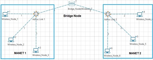
Bridge Node#
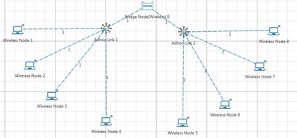
Bridge Node acts as a bridge/interface/gateway between multiple MANETs. Packets from one MANET can be routed to another MANET via a Bridge Node as shown Figure
Each Bridge Node has 24 interfaces. When connecting bridge nodes to one another or to routers care should be taken to ensure that the static routes are set. This is required since the bridge nodes do not run any routing protocol.
NetSim supports Wired and Wireless Bridge nodes as shown Figures.
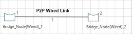

A wired bridge node cannot be connected to a wireless bridge node and vice versa
Adhoc Link#
At a given point in time, depending on the nodes' positions and their transmitter and receiver coverage patterns, transmission power levels and interference levels, a wireless connectivity in the form of a random, multihop graph or "ad hoc" network exists between the nodes. This ad hoc topology may change with time as the nodes move or adjust their transmission and reception parameters. Ad hoc links are used in NetSim to visually represent this connection of devices in an Ad hoc basis as shown in below Figure.

Wireless links generally have significantly lower capacity than their hardwired counterparts. In addition, the realized throughput of wireless communications after accounting for the effects of multiple access, fading, noise, and interference conditions, etc. is often much less than a radio's maximum transmission rate.
Connecting Adhoc links is a two-step process.
- Click and drop the Adhoc link icon from the device panel.
- Click (select) the Adhoc link, from the ribbon (toolbar). Then click on a wireless node and on the dropped adhoc link icon (on grid). This will connect the wireless node to the adhoc link.
- The connection between wireless nodes and adhoc link (icon on grid) is not to be done using a wireless link but using an Adhoc link (in ribbon) itself.
Single MANETs#
A sample single MANET scenario comprises of only wireless nodes without any bridge node. It would look as shown below Figure.

Multiple MANETs#
Multiple MANETs allows users to interconnect two or more MANETs using a bridge node.Select “Manually via Click and Drop” option in the Mobile Adhoc Networks fast config window as shown below and click on OK button as shown in below Figure

Click and drop Wireless nodes, Adhoc links and Bridge Node onto the grid environment

Click on Adhoc Link icon (in ribbon). Then click on adhoc link icon (in grid) and on Wireless node (in grid) to connect Adhoc link to Wireless Node. Similarly connect Wireless Nodes to Adhoc links to form two different MANET’s using Adhoc links. Further connect the two MANET’s using a bridge node as shown below Figure.
Multiple MANETs do not support DSR, OLSR and ZRP protocols which is available in single MANETs
Set Node, Link and Application Properties#
Right click on the appropriate node or link and select Properties. Then modify the parameters according to the requirements.
- Global Properties: Certain properties are global in nature, i.e., changing properties in one node will automatically reflect in the others in that network.
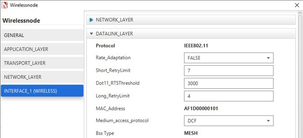
- In case of MANET, in Wireless Node, Routing Protocol in Network Layer is global and all user editable properties in Datalink Layer, Physical Layer and Power are Local.
- The following are the main properties of wireless node in Datalink and Physical layers as shown in below Figures.


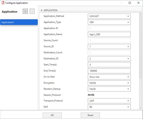
- Click on the Application icon present on the ribbon and set properties. Multiple applications can be generated by using “+” button in Application properties.
- Set the values according to requirement and click OK.
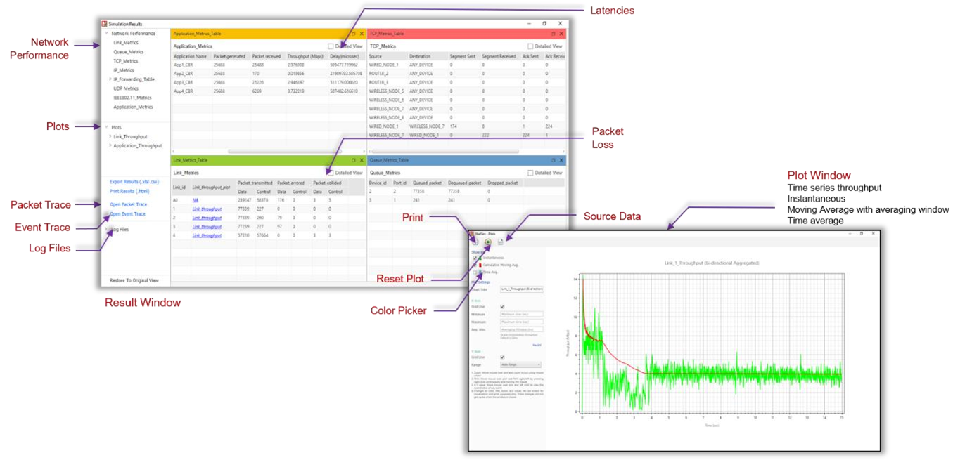
Enable Packet Trace, Event Trace & Plots (Optional)#
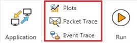
Click Packet Trace / Event Trace icon in the tool bar and check Enable Packet Trace / Event Trace check box and click OK. To get detailed help, please refer sections 8.4and 8.5 in User Manual. Select Plots icon for enabling Plots and click OK.
Run Simulation#
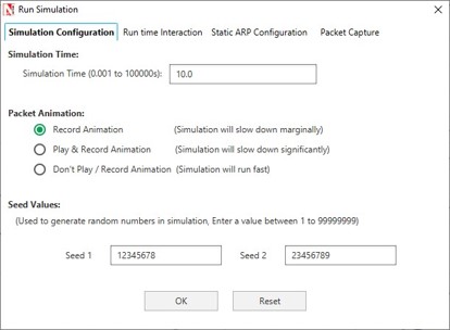
- Click on Run Simulation icon on the top toolbar
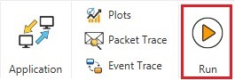
- Set the Simulation Time and click on OK.
Note on MANET implementation in NetSim
- If user wants to implement HTTP application among Nodes, TCP must be enabled in Source Node as TCP is set to disable by default.
- OLSR is a proactive link-state routing protocol, which uses Hello and topology control (TC) messages to discover and then disseminate link state information throughout the mobile ad hoc network.
- Individual nodes use this topology information to compute next hop destinations for all nodes in the network using shortest hop forwarding paths. For topology control (TC) messages to disseminate throughout, it requires 5 or more seconds depending upon the network size. In general, it is (5.5 secs + Tx_Time * network size).
- Hence, when simulating OLSR in MANET the Application Start Time must be greater than 5s (preferably greater than 10s) because in OLSR Topology Control (TC) messages start at 5s. Once the TC messages are sent, some further time will be required for OLSR to find the route. This can be done by setting the “Start_Time” parameter in Application properties
Model Features#
Adhoc On Demand Distance Vector Routing#
The Ad hoc On-Demand Distance Vector (AODV) algorithm enables dynamic, self-starting, multihop routing between participating mobile nodes wishing to establish and maintain an ad hoc network. AODV allows mobile nodes to respond to link breakages and changes in network topology in a timely manner. When links break, AODV causes the affected set of nodes to be notified so that they can invalidate the routes using the lost link. AODV in NetSim can run in layer 3 over MAC/PHY protocols such as 802.11, 802.15.4, TDMA and DTDMA.
The features of AODV implemented in NetSim are:
Broadcast Route Discovery Mechanism, and Route Maintenance: AODV accomplishes this with the help of RREQ AND RREP. The packet trace file and the packet animation window in NetSim help to view and understand how AODV accomplishes this mechanism using RREQ and RREP packets.
Timer - based states: Routing table states expire when the route remains inactive for a certain period of time. This is established by the use of the lifetime field in the routing table and RREP packets. The lifetime field can be viewed in Wireshark under the AODV RREP packets.
Sequence numbers: The source sequence number is a monotonically increasing number maintained by each source node. It is used by other nodes to determine whether the information contained in the packet send by the source node is new. The destination sequence number is created by destination to be included with the routing information that it sends to the requesting nodes. Usage of destination sequence number ensures loop freedom. The route with the greatest sequence number is used by requesting node to reach destination. This also prevents routing loops and avoid using inactive or old routes. The source and destination sequence numbers can be viewed in Wireshark under the RREQ and RREP packets in AODV protocols.
Some important fields of the RREQ format that can be viewed in NetSim using Wireshark are mentioned below Table
| Hop Count | The number of hops from the Originator IP Address to the node handling the request. |
|---|---|
| Destination IP Address | The IP address of the destination for which a route is desired. |
| Destination Sequence Number | The latest sequence number received in the past by the originator for any route towards the destination. |
| Originator IP Address | The IP address of the node which originated the Route Request. |
| Originator Sequence Number | The current sequence number to be used in the route entry pointing toward the originator node. |
Some important fields of the RREP format that can be viewed in NetSim using Wireshark are mentioned below Table.
| Hop count | The number of hops from the Originator IP Address to the Destination IP Address. |
|---|---|
| Destination IP Address | The IP address of the destination for which a route is supplied. |
| Destination Sequence Number | The destination sequence number associated to the route |
| Originator IP Address | The IP address of the node which send the RREQ. |
| Lifetime | The time in milliseconds for which nodes receiving the RREP consider the route to be valid. |
Dynamic Source Routing (DSR)#
The Dynamic Source Routing protocol (DSR) is a simple and efficient routing protocol designed specifically for use in multi-hop wireless ad-hoc networks of mobile nodes. Using DSR, the network is completely self-organizing and self-configuring, requiring no existing network infrastructure or administration. Network nodes cooperate to forward packets for each other to allow communication over multiple "hops" between nodes not directly within wireless transmission range of one another. As nodes in the network move about or join or leave the network, and as wireless transmission conditions such as sources of interference change, all routing is automatically determined and maintained by the DSR routing protocol. Since the number or sequence of intermediate hops needed to reach any destination may change at any time, the resulting network topology may be quite rich and rapidly changing. DSR in NetSim can run in layer 3 over MAC/PHY protocols such as 802.11, 802.15.4, TDMA and DTDMA.
Using Link-Layer Acknowledgements#
If the MAC protocol in use provides feedback as to the successful delivery of a data packet (such as is provided for unicast packets by the link-layer acknowledgement frame defined by IEEE 802.11), then the use of the DSR Acknowledgement Request and Acknowledgement options is not necessary. If such link-layer feedback is available, it SHOULD be used instead of any other acknowledgement mechanism for Route Maintenance, and the node SHOULD NOT use either passive acknowledgements or network-layer acknowledgements for Route Maintenance.When using link-layer acknowledgements for Route Maintenance, the retransmission timing and the timing at which retransmission attempts are scheduled are generally controlled by the particular link layer implementation in use in the network. For example, in IEEE 802.11, the link-layer acknowledgement is returned after a unicast packet as a part of the basic access method of the IEEE 802.11 Distributed Coordination Function (DCF) MAC protocol; the time at which the acknowledgement is expected to arrive and the time at which the next retransmission attempt (if necessary) will occur are controlled by the MAC protocol implementation.
Using Network-Layer Acknowledgements#
When a node originates or forwards a packet and has no other mechanism of acknowledgement available to determine reachability of the next-hop node in the source route for Route Maintenance, that node SHOULD request a network-layer acknowledgement from that next-hop node. To do so, the node inserts an Acknowledgement Request option in the DSR Options header in the packet. The Identification field in that Acknowledgement Request option MUST be set to a value unique over all packets recently transmitted by this node to the same next-hop node.
When using network-layer acknowledgements for Route Maintenance, a node SHOULD use an adaptive algorithm in determining the retransmission timeout for each transmission attempt of an acknowledgement request. For example, a node SHOULD maintain a separate round-trip time (RTT) estimate for each node to which it has recently attempted to transmit packets, and it should use this RTT estimate in setting the timeout for each retransmission attempt for Route Maintenance.
While simulating certain network configurations, users may see that packets received are more than packets sent. This is because:
- This is being measured as part of our UDP protocol metrics in layer 4 in the source and in the destination.
- Let us say UDP protocol at source node A sends a datagram. At the MAC - WLAN send the frame and starts a re-transmission timer.
- If no Ack is received within this timer period it would initiate a re-transmission (consider cases where the WLAN Ack has a collision or is errored).
- As the destination the MAC (WLAN) layer would send up to UDP both the first packet it received and the re-transmitted packet it received.
- UDP protocol in the destination would count both the packets received

Who do we see continuous RREQ and RREP packets in DSR?#
When the Data packet are to be transmitted, in DSR, within the NETWORK_OUT Event, the DSR-packet-processing function is called. This initiates Route discovery, if no route to destination exists. Once discovery is complete, DSR switches to Route maintenance mode.
Route Maintenance is the mechanism by which a source node S is able to detect, while using a source route to some destination node D, if the network topology has changed such that it can no longer use its route to D because a link along the route no longer works.
In Route Maintenance mode, DSR checks for ACKs for every data packet sent. If the ACK for a data packet, is not received within a specified time (as defined by the Maintenance Time Out) then Route Error (RERR) gets triggered. This trigger leads removal of Route entries from the Route Cache thereby causing Route discovery to be initiated again.
A typical simulation scenario where Route discovery, Router error, Route discovery, Router Error cycle is repeated, is when the network has multiple applications generate data packets at the exact same time. This can cause packet collisions in the MAC layer. Since no packet is received no ACK is sent. The non-receipt of ACK within the specified time causes RERR to get triggered
AODV/DSR Metrics#
AODV or DSR Metrics table will be part of the results dashboard if routing protocol in the network layer is set to either AODV or DSR in at least one device in the network scenario simulated.
| Parameter | Description |
|---|---|
| Device Id | It is the unique ID of the wireless node |
| RREQ sent | It is the number of Route Request packets sent by wireless node during Route Discovery process |
| RREQ forwarded | It is the number of Route Request packets forwarded by wireless node during Route Discovery process |
| RREP sent | It is the number of Route Reply packets sent by wireless node when route is found during Route Discovery process |
| RREP forwarded | It is the number of Route Reply packets forwarded by a wireless node when route is found during Route Discovery process |
| RERR sent | It is the total number of Route Error packets sent by a wireless node during Route Maintenance |
| RERR forwarded | It is the total number of Route Error packets forwarded by a wireless node during Route Maintenance |
| Packet originated | It is the total number of packets originated in a source node |
| Packet transmitted | It is the total number of packets transmitted by a source node and intermediate device (LoWPAN Gateway or sink node) |
| Packet dropped | It is the total number of packets dropped by a wireless node |
Zone Routing Protocol (ZRP)#
The ZRP is based on two procedures:
- Intrazone Routing Protocol (IARP) and
- Interzone Routing Protocol (IERP).
Through the use of the IARP, each node learns the identity of and the (minimal) distance to all the nodes in its routing zone. The actual IARP is not specified and can include any number of protocols, such as the derivatives of Distance Vector Protocol (e.g., Ad Hoc On-Demand Distance Vector, Shortest Path First (e.g., OSPF). In fact, different portions of an ad hoc network may choose to operate based on different choice of the IARP protocol. Whatever the choice of IARP is, the protocol needs to be modified to ensure that the scope of this operation is restricted to the zone of the node in question.
Note that as each node needs to learn the distances to the nodes within its zone only, the nodes are updated about topological changes only within their routing zone. Consequently, inspite of the fact that a network can be quite large, the updates are only locally propagated.
IERP
While IARP finds routes within a zone, IERP is responsible for finding routes between nodes located at distances larger than the zone radius. IERP relies on border casting. Border casting is possible as any node knows the identity and the distance to all the nodes in its routing zone by the virtue of the IARP protocol.
The IERP operates as follows: The source node first checks whether the destination is within its routing zone. (Again, this is possible as every node knows the content of its zone). If so, the path to the destination is known and no further route discovery processing is required. If, on the other hand, the destination is not within the source's routing zone, the source border casts a route request (referred to here as a "request") to all its peripheral nodes. Now, in turn, all the peripheral nodes execute the same algorithm: check whether the destination is within their zone. If so, a route reply (referred to here as a "reply") is sent back to the source indicating the route to the destination. If not, the peripheral node forwards the query to its peripheral nodes, which, in turn, execute the same procedure. An example of this Route Discovery procedure is demonstrated in the figure below Figure
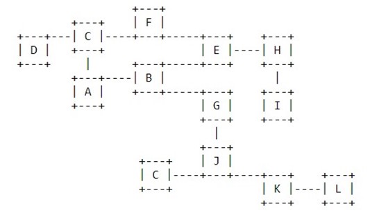
The node A has a datagram to node L. Assume routing zone radius of 2. Since L is not in A's routing zone (which includes B, C, D, E, F, G), A border cast a routing request to its peripheral nodes: D, F, E, and G. Each one of these peripheral nodes check whether L exists in their routing zones. Since L is not found in any routing zones of these nodes, the nodes border cast the request to their peripheral nodes. In particular, G border casts to K, which realizes that L is in its routing zone and returns the requested route (L-K-G-A) to the query source, namely A.
IARP
In Zone Routing, the Intrazone Routing Protocol (IARP) proactively maintains routes to destinations within a local neighborhood, which we refer to as a routing zone. More precisely, a node's routing zone is defined as a collection of nodes whose minimum distance in hopsfrom the node in question is no greater than a parameter referred to as the zone radius. Note that each node maintains its own routing zone. An important consequence is that the routing zones of neighboring nodes overlap.
An example of a routing zone (for node A) of radius 2 is shown below Figure

Note that in this example nodes B through F are within the routing zone of A. Node G is outside A's routing zone. Also note that E can be reached by two paths from A, one with length 2 hops and one with length 3 hops. Since the minimum is less or equal than 2, E is within A's routing zone.
Peripheral nodes are nodes whose minimum distance to the node in question is equal exactly to the zone radius. Thus, in the above figure, nodes D, F, and E are A's peripheral nodes.
The construction of a routing zone requires a node to first know who its neighbors are. A neighbor is defined as a node with whom direct (point-to-point) communication can be established and is, thus, one hop away. Identification of a node's neighbors may be provided directly by the media access control (MAC) protocols, as in the case of polling-based protocols. In other cases, neighbor discovery may be implemented through a separate Neighbor Discovery Protocol (NDP). Such a protocol typically operates through the periodic broadcasting of "hello" beacons. The reception (or quality of reception) of a "hello" beacon can be used to indicate the status of a connection to the beaconing neighbor.Neighbor discovery information is used as a basis for the IARP. IARP can be derived from globally proactive link state routing protocols that provide a complete view of network connectivity
Optimized Link State Routing Protocol (OLSR)#
OLSR is developed for mobile ad hoc networks. It operates as a table driven, proactive protocol, i.e., exchanges topology information with other nodes of the network regularly. Each node selects a set of its neighbor nodes as "multipoint relays" (MPR). In OLSR, only nodes, selected as such MPRs, are responsible for forwarding control traffic, intended for diffusion into the entire network. MPRs provide an efficient mechanism for flooding control traffic by reducing the number of transmissions required.
Nodes, selected as MPRs, also have a special responsibility when declaring link state information in the network. Indeed, the only requirement for OLSR to provide shortest path routes to all destinations is that MPR nodes declare link-state information for their MPR selectors. Additional available link-state information may be utilized, e.g., for redundancy.
Nodes which have been selected as multipoint relays by some neighbor node(s) announce this information periodically in their control messages. Thereby a node announces to the network, that it has reachability to the nodes which have selected it as an MPR. In route calculation, the MPRs are used to form the route from a given node to any destination in the network. Furthermore, the protocol uses the MPRs to facilitate efficient flooding of control messages in the network.
Neighbor detection#
Neighbor detection populates the neighborhood information base and concerns itself with nodes and node main addresses. The mechanism for neighbor detection is the periodic exchange of HELLO messages.
A node maintains a set of neighbor tuples, based on the link tuples. This information is updated according to changes in the Link Set. The Link Set keeps the information about the links, while the Neighbor Set keeps the information about the neighbors. There is a clear association between those two sets, since a node is a neighbor of another node if and only if there is at least one link between the two nodes.
The "Originator Address" of a HELLO message is the main address of the node, which has emitted the message. Upon receiving a HELLO message, a node SHOULD first update its Link Set and then update its Neighbor Set.
Topology discovery#
The link sensing and neighbor detection part of the protocol basically offers, to each node, a list of neighbors with which it can communicate directly and, in combination with the Packet Format and Forwarding part, an optimized flooding mechanism through MPRs. Based on this, topology information is disseminated through the network.
TC message#
In order to build the topology information base, each node, which has been selected as MPR, broadcasts Topology Control (TC) messages. TC messages are flooded to all nodes in the network and take advantage of MPRs. MPRs enable a better scalability in the distribution oftopology information.
The list of addresses can be partial in each TC message (e.g., due to message size limitations, imposed by the network), but parsing of all TC messages describing the advertised link set of a node MUST be complete within a certain refreshing period (TC_INTERVAL). The information diffused in the network by these TC messages will help each node calculate its routing table.
When the advertised link set of a node becomes empty, this node SHOULD still send (empty) TC-messages during the duration equal to the "validity time" (typically, this will be equal to TOP_HOLD_TIME) of its previously emitted TC-messages, in order to invalidate the previous TC-messages. It SHOULD then stop sending TC-messages until some node is inserted in its advertised link set.
A node MAY transmit additional TC-messages to increase its reactiveness to link failures. When a change to the MPR selector set is detected and this change can be attributed to a link failure, a TC-message SHOULD be transmitted after an interval shorter than TC_INTERVAL.
Mobility models in NetSim#
Mobility models represent the movement of mobile user, and how their location, velocity and acceleration change over time. Such models are frequently used for simulation purposes when new communication or navigation techniques are investigated, or to evaluate the performance of mobile wireless systems and the algorithms and protocols at the basis of them.
The movement of all nodes in NetSim is logged in the Animation_Node_Movement.txt file (if animation is enabled). This file will get saved to the same folder where the experiment is saved. Upon examining the file one can note that the node movement calculations are done every Calculation_Interval.
The mobility models provided in NetSim are as follows
Random Walk Mobility Model#
It is a simple mobility model based on random directions and speeds. In this mobility model, a mobile node moves from its current location to a new location by randomly choosing a direction and speed in which to travel. The new speed and direction are both chosen from pre-defined ranges. Each movement in the Random Walk Mobility Model occurs in either a constant time interval or a constant distance traveled, at the end of which a new direction and speed are calculated.
Random Waypoint Mobility Model#
It includes pause time between changes in direction and/or speed. A mobile node begins by staying in one location for a certain period of time (i.e., a pause time). Once this time expires, the mobile node chooses a random destination in the simulation area and a speed that is uniformly distributed between [minspeed, maxspeed]. The mobile node then travels toward the newly chosen destination at the selected speed. Upon arrival, the mobile node pauses for a specified PauseTime before starting the process again. Note that the movement calculation is done every Calculation_Interval. Therefore, it is recommended to set the PauseTime as an integral multiple of Calculation_Interval.
Group Mobility Model#
It is a model which describes the behavior of mobile nodes as they move together i.e. the devices having common group id will move together.
Pedestrian Mobility Model#
This model is applicable to each node (local parameter), and the configuration parameters are:
- Pedestrian_Max_Speed (m/s) (Range: 0.0 to 10.0. Default: 3.0)
- Pedestrain_Min_Speed (m/s) (Range: 0.0 to 10.0. Default: 1.0)
- Pedestrian_stop_probability (Range: 0 to 1)
- Pedestrian_stop_duration (s). (Range: 1 to 10000)
In this model it is assume that the pedestrian stops at traffic lights. The stop_probability represents the probability of encountering a traffic light. This is checked for every Calcuation_interval. Once stopped, the pedestrian waits for a duration equal to stop_duration for the light to turn green. A new direction is chosen randomly after every stop with 𝜃 (angle between new direction and current direction) taking values of 0, 90, 180, 270. These 𝜃 values represent the pedestrian continuing in the same direction, taking a left, taking a U turn and taking a right respectively.
A new speed is chosen randomly after evert stop. $Min_speed ≤ 𝑆𝑝𝑒𝑒𝑑 ≤ Max_Speed$
The maximum number of stops and starts is 10.
File Based Mobility Model#
In File Based Mobility, users can write their own custom mobility models and define the movement of the mobile users. The content should be per the NetSim Mobility File format explained below. The user can also generate the mobility files using external tools like SUMO (Simulation of Urban Mobility), Vanet MobiSim etc.
The NetSim Mobility File setting and format is explained below:
Step 1: Right click to open Properties of Wireless_Node (MANET) or UE (LTE Networks). Then properties -> General Properties -> select mobility model as File_Based_Mobility and click on Open Mobility file.
Step 2: Inside the text file and write the node mobility in format shown below.
#To write comments, use # tag
#Specify the new location of the specific device at the specific time
$time <Time_in_Secs> "$node (<Node_ID - 1>) <X_Coordinate><Y_Coordinate ><Z_Coordinate >"
A sample file-based mobility experiment is present at <NetSim Installed Directory>\Docs\Sample_Configuration\ MANET.
A sample mobility.txt file for a MANET network containing 2 nodes is shown below.
$time 0.0 "$node_(0) 70.00 70.00 0.00"
$time 0.0 "$node_(1) 150.0 150.0 0.0"
$time 5.0 "$node_(0) 100.00 70.00 0.00"
$time 5.0 "$node_(1) 150.0 160.0 0.0"
$time 10.0 "$node_(0) 130.00 70.00 0.00"
$time 10.0 "$node_(1) 150.0 170.0 0.0"
$time 15.0 "$node_(0) 160.00 70.00 0.00"
$time 15.0 "$node_(1) 150.0 180.0 0.0"
$time 20.0 "$node_(0) 190.00 70.00 0.00"
$time 20.0 "$node_(1) 150.0 190.0 0.0"
$time 25.0 "$node_(0) 220.00 70.00 0.00"
$time 25.0 "$node_(1) 150.0 200.0 0.0"
$time 30.0 "$node_(0) 250.00 70.00 0.00"
$time 30.0 "$node_(1) 150.0 210.0 0.0"
$time 35.0 "$node_(0) 280.00 70.00 0.00"
$time 35.0 "$node_(1) 150.0 220.0 0.0"
$time 40.0 "$node_(0) 310.00 70.00 0.00"
$time 40.0 "$node_(1) 150.0 230.0 0.0"
$time 45.0 "$node_(0) 340.00 70.00 0.00"
$time 45.0 "$node_(1) 150.0 240.0 0.0"
$time 50.0 "$node_(0) 370.00 70.00 0.00"
$time 50.0 "$node_(1) 150.0 250.0 0.0"
Note: NetSim does not interpolate device mobility between two entries in the mobility file. This means that in the simulation the device “jumps” to the next point at that instant in time. The mobility is not “continuous” from one point to another over time.
Visualizing node movement in NetSim Animator#
NetSim animator animates the flow of packets in the network along with device mobility if configured. Viewing of node movement in NetSim animator is impacted by:
- Time Units: movement is based on update interval which by default is set to 1 second in the UI. In case of file-based mobility, for example there are movement entries at 1.25 seconds and 1.5 seconds. However, the animator progresses time in the order of microseconds. This sometimes means that users would need to wait for a long time to view node movement.
- Application start time: It is generally set to 5s but can be set to other values. Packet generation will start only at the application start time.
- Grid size: If the grid size is set in thousands of meters whereas the movement of the devices is only in tens of meters then movement may not be visible even though it is happening.
- Relation between time set in mobility file and time set for simulation: In case of File Based Mobility where a movements file (mobility.txt) is provided as input to NetSim, if the mobility file contains entries beyond the simulation time, only those entries that lie within the simulation start and end time will be considered for the simulation and corresponding movement can be viewed in the animation.
- Channel characteristics: If the devices communicating in the network aren't within the range of one another or if there is no successful data transmission in the network during the simulation, animation may not show any device movement
How are packet collisions modelled in NetSim?#
Packet Collision is a theoretical concept. In the real world, a packet is not a "physical" entity that can collide. Therefore a "collision" is the interference of two radio waves (of the packets being sent).
In NetSim the collision model is as follows:
- At the transmitter, when a packet is being transmitted, if the sum of received power from all other nodes is greater than the receiver sensitivity then that packet is marked as collided.
- At the receiver, when a packet is being received, if the sum of the received power from all other nodes, except the node from where this packet is being transmitted, is greater than the receiver sensitivity then that packet is marked as collided.
- There is also a special case where a Single Packet can be marked as collided as explained below:
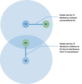
Where, T1 and T2 are transmitters.
R1 and R2 are receivers.
How is packet error decided in NetSim#
The way the packet error is decided is given as follows:
- Compute Rx power at the receiver based on Tx Power, fewer losses due to Propagation. Propagation models cover HATA Urban, Sub Urban, COST 231 HATA, Indoor Home / Office, Factory, Lognormal, Friis Free space. Apart from path loss, fading and shadowing can also be modeled.
- Rx Power / (Background Noise + Interference noise) = SINR. Here Interference noise is due to other transmissions within the network.
- Based on the SINR, BER is got from the respective modulation curve/table.
- Based on the BER, the packet error rate is decided
- NetSim does not perform bit-wise simulation since it would be too computationally intensive.
Broadcast and Multicast in MANETs#
In MANET, only neighbour (nodes within transmission range) broadcast/multicast is supported; multi-hop broadcast/ multicast is not supported. This means that nodes that are 2-hops or more away will not receive the broadcast packets. The reason for not implementing multi-hop broadcast/multicast is explained below.
The simplest form of broadcast in an ad hoc network is where a node transmits a broadcast packet, which is received by all neighboring nodes that are within transmission range. Upon receiving a broadcast packet, each node determines if it has transmitted the packet before. If not, then the packet is retransmitted. This process allows for a broadcast packet to be disseminated throughout the ad hoc network. The process terminates when all nodes have received and transmitted the packet being broadcast at least once.
This method of broadcasting is required given the dynamic nature of ad hoc networks, i.e., nodes move around, and neighbors may change as the broadcast is happening. Now, since all nodes participate in the broadcast, its causes flooding and hence suffers from the Broadcast Storm Problem. Flooding is extremely costly and leaves the network completely congested. Special algorithms are required to alleviate the broadcast storm problem. Custom development will be required to implement them.
Featured Examples#
- AODV-ROUTING
- ZRP-IARP
- ZRP-IERP
- MANET-OLSR
- MULTIPLE-MANET
- Power Models in MANET
- Application throughput variation with node mobility
Reference Documents#
- IEEE 802.11 - 2012 Standard for Wireless LAN
- AODV – RFC 3561
- OLSR – RFC 3626
- ZRP – Draft RFC Zone ZRP
- MANET Routing protocol performance issues - RFC 2501
Latest FAQs#
Up to date FAQs on NetSim’s MANET library is available at https://tetcos.freshdesk.com/support/solutions/folders/14000110331