Study the working and routing table formation of Interior routing protocols, i.e. Routing Information Protocol (RIP) and Open Shortest Path First (OSPF)
Introduction#
RIP#
RIP is intended to allow hosts and gateways to exchange information for computing routes through an IP-based network. RIP is a distance vector protocol which is based on Bellman-Ford algorithm. This algorithm has been used for routing computation in the network.
Distance vector algorithms are based on the exchange of only a small amount of information using RIP messages.
Each entity (router or host) that participates in the routing protocol is assumed to keep information about all of the destinations within the system. Generally, information about all entities connected to one network is summarized by a single entry, which describes the route to all destinations on that network. This summarization is possible because as far as IP is concerned, routing within a network is invisible. Each entry in this routing database includes the next router to which datagram's destined for the entity should be sent. In addition, it includes a \"metric\" measuring the total distance to the entity.
Distance is a somewhat generalized concept, which may cover the time delay in getting messages to the entity, the dollar cost of sending messages to it, etc. Distance vector algorithms get their name from the fact that it is possible to compute optimal routes when the only information exchanged is the list of these distances. Furthermore, information is only exchanged among entities that are adjacent, that is, entities that share a common network.
OSPF#
In OSPF, the Packets are transmitted through the shortest path between the source and destination.
OSPF allows administrator to assign a cost for passing through a link. The total cost of a particular route is equal to the sum of the costs of all links that comprise the route. A router chooses the route with the shortest (smallest) cost.
In OSPF, each router has a link state database which is tabular representation of the topology of the network (including cost). Using Dijkstra algorithm each router finds the shortest path between source and destination.
Formation of OSPF Routing Table#
-
OSPF-speaking routers send Hello packets out all OSPF-enabled interfaces. If two routers sharing a common data link agree on certain parameters specified in their respective Hello packets, they will become neighbors.
-
Adjacencies, which can be thought of as virtual point-to-point links, are formed between some neighbors. OSPF defines several network types and several router types. The establishment of an adjacency is determined by the types of routers exchanging Hellos and the type of network over which the Hellos are exchanged.
-
Each router sends link-state advertisements (LSAs) over all adjacencies. The LSAs describe all of the router\'s links, or interfaces, the router\'s neighbors, and the state of the links. These links might be to stub networks (networks with no other router attached), to other OSPF routers, or to external networks (networks learned from another routing process). Because of the varying types of link-state information, OSPF defines multiple LSA types.
-
Each router receiving an LSA from a neighbor records the LSA in its link-state database and sends a copy of the LSA to all of its other neighbors.
-
By flooding LSAs throughout an area, all routers will build identical link-state databases.
-
When the databases are complete, each router uses the SPF algorithm to calculate a loop-free graph describing the shortest (lowest cost) path to every known destination, with itself as the root. This graph is the SPF tree.
-
Each router builds its route table from its SPF tree.
Network Setup#
Open NetSim and click on Experiments> Internetworks> Routing and Switching> Route table formation in RIP and OSPF then click on the tile in the middle panel to load the example as shown in below Figure 16‑1.

Figure 16‑1: List of scenarios for the example of Route table formation in RIP and OSPF
NetSim UI displays the configuration file corresponding to this experiment as shown below Figure 16‑2.

Figure 16‑2: Network set up for studying the RIP/OSPF
Procedure#
[RIP]{.underline}
The following are the set of procedures were done to generate this sample.
Step 1: A network scenario is designed in the NetSim GUI comprising of 2 Wired Nodes, 2 L2 Switches, and 7 Routers.
Step 2: Go to Router 1 Properties. In the Application Layer, Routing Protocol is set as RIP Figure 16‑3.

Figure 16‑3: Application Layer Window - Routing Protocol is set as RIP
The Router Configuration Window shown above, indicates the Routing Protocol set as RIP along with its associated parameters. The "Routing Protocol" parameter is Global. i.e., changing in Router 1 will affect all the other Routers. So, in all the Routers, the Routing Protocol is now set as RIP.
Step 3: Right click on App1 CUSTOM and select Properties or click on the Application icon present in the top ribbon/toolbar. Transport Protocol is set to UDP.
A CUSTOM Application is generated from Wired Node 10 i.e., Source to Wired Node 11 i.e., Destination with Packet Size remaining 1460Bytes and Inter Arrival Time remaining 20000µs.
Step 4: Packet Trace is enabled, and hence we are able to track the route which the packets have chosen to reach the destination based on the Routing Information Protocol that is set.
Step 5: Enable the plots and run the Simulation for 100 Seconds.
[OSPF]{.underline}
The following are the set of procedures that are followed to carry out this experiment.
Step 1: A network scenario is designed in the NetSim GUI comprising of 2 Wired Nodes, 2 L2 Switches, and 7 Routers.
Step 2: Go to Router 1 Properties. In the Application Layer, Routing Protocol is set as OSPF Figure 16‑4.

Figure 16‑4: Application Layer Window - Routing Protocol is set as OSPF
The Router Configuration Window shown above, indicates the Routing Protocol set as OSPF along with its associated parameters. The "Routing Protocol" parameter is Global. i.e., changing in Router 1 will affect all the other Routers. So, in all the Routers, the Routing Protocol is now set as OSPF.
Step 3: Go to Router 7 Properties. In both the WAN Interfaces, the Output Cost is set to 2000 Figure 16‑5.
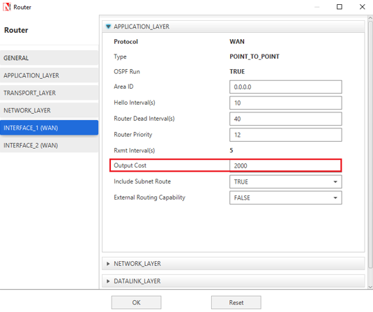
Figure 16‑5: WAN Interfaces- Output Cost is set to 2000
The "Output Cost" parameter in the WAN Interface > Application Layer of a router indicates the cost of sending a data packet on that interface and is expressed in the link state metric.
Step 4: Right click on App1 CUSTOM and select Properties or click on the Application icon present in the top ribbon/toolbar.
A CUSTOM Application is generated from Wired Node 10 i.e., Source to Wired Node 11 i.e., Destination with Packet Size remaining 1460Bytes and Inter Arrival Time remaining 20000µs.
Additionally, the "Start Time (s)" parameter is set to 40, while configuring the application. This time is usually set to be greater than the time taken for OSPF Convergence (i.e., Exchange of OSPF information between all the routers), and it increases as the size of the network increases.
Step 5: Packet Trace is enabled, and hence we are able to track the route which the packets have chosen to reach the destination based on the Open Shortest Path First Routing Protocol that is set.
Step 6: Enable the plots and run the Simulation for 100 Seconds.
Output for RIP#
Go to NetSim Packet Animation window and play the animation. The route taken by the packets to reach the destination can be seen in the animation as well as in the below table containing various fields of packet information as shown below Figure 16‑6.

Figure 16‑6: Animation window for RIP
Users can view the same in Packet Trace.
Shortest Path from Wired Node 10 to Wired Node 11 in RIP is Wired Node 10->L2 Switch 8->Router 1->Router 7->Router 6->L2 Switch 9->Wired Node 11. RIP chooses the lower path (number of hops is less) to forward packets from source to destination, since it is based on hop count.
Output for OSPF#
Go to NetSim Packet Animation window and play the animation. The route taken by the packets to reach the destination can be seen in the animation as well as in the below table containing various fields of packet information as shown below Figure 16‑7.

Figure 16‑7: Animation window for OSPF
Users can view the same in Packet Trace.
Shortest Path from Wired Node 10 to Wired Node 11 in OSPF (Use Packet Animation to view) Wired Node 10->L2 Switch 8->Router 1->Router 2->Router 3->Router 4->Router 5->Router 6->L2 Switch 9->Wired Node 11. OSPF chooses the above path (cost is less-5) since OSPF is based on cost.
Inference#
RIP#
In Distance vector routing, each router periodically shares its knowledge about the entire network with its neighbors. The three keys for understanding the algorithm,
-
Knowledge About The Whole Network - Router sends all of its collected knowledge about the network to its neighbors.
-
Routing Only To Neighbors - Each router periodically sends its knowledge about the network only to those routers to which it has direct links. It sends whatever knowledge it has about the whole network through all of its ports. This information is received and kept by each neighboring router and used to update it's own information about the network.
-
Information Sharing At Regular Intervals - For example, every 30 seconds, each router sends its information about the whole network to its neighbors. This sharing occurs whether or not the network has changed since the last time, information was exchanged
In NetSim the Routing Table Formation has 3 stages,
-
Initial Table: The Initial Table will show the direct connections made by each Router.
-
Intermediate Table: The Intermediate Table will have the updates of the Network in every 30 seconds.
-
Final Table: The Final Table is formed when there is no update in the Network.
The data should be forwarded using Routing Table with the shortest distance.
OSPF#
The main operation of the OSPF protocol occurs in the following consecutive stages, and leads to the convergence of the internetworks:
-
Compiling the LSDB.
-
Calculating the Shortest Path First (SPF) Tree.
-
Creating the routing table entries.
Compiling the LSDB
The LSDB is a database of all OSPF router LSAs. The LSDB is compiled by an ongoing exchange of LSAs between neighboring routers so that each router is synchronized with its neighbor. When the Network converged, all routers have the appropriate entries in their LSDB.
Calculating the SPF Tree Using Dijkstra\'s Algorithm
Once the LSDB is compiled, each OSPF router performs a least cost path calculation called the Dijkstra algorithm on the information in the LSDB and creates a tree of shortest paths to each other router and network with themselves as the root. This tree is known as the SPF Tree and contains a single, least cost path to each router and in the Network. The least cost path calculation is performed by each router with itself as the root of the tree.
Calculating the Routing Table Entries from the SPF Tree
The OSPF routing table entries are created from the SPF tree and a single entry for each network in the AS is produced. The metric for the routing table entry is the OSPF-calculated cost, not a hop count.
If the application start time isn\'t changed then,
-
Packets generated before OSPF table convergence may be dropped at the gateway router.
-
The application may also stop if ICMP is enabled in the router.
-
If TCP is enabled TCP may stop after the re-try limit is reached (since the SYN packets would not reach the destination)
NOTE: The device / link numbering and IP Address setting in NetSim is based on order in which in the devices are dragged & dropped, and the order in which links are connected. Hence if the order in which a user executes these tasks is different from what is shown in the screen shots, users would notice different tables from what is shown in the screen shots.