Performance Evaluation of a Star Topology IoT Network
Introduction#
In IOT experiments 20 and 21 we studied a single IoT device connected to a sink (either directly or via IEEE 802.15.4 routers). Such a situation would arise in practice, when, for example, in a large campus, a ground level water reservoir has a water level sensor, and this sensor is connected wirelessly to the campus wireline network. Emerging IoT applications will require several devices, in close proximity, all making measurements on a physical system (e.g., a civil structure, or an industrial machine). All the measurements would need to be sent to a computer connected to the infrastructure for analysis and inferencing. With such a scenario in mind, in this experiment, we will study the performance of several IEEE 802.15.4 devices each connected by a single wireless link to a sink. This would be called a "star topology" as the sensors can be seen as the spikes of a "star."
We will set up the experiment such that every sensor can sense the transmissions from any other sensor to the sink. Since there is only one receiver, only one successful transmission can take place at any time. The IEEE 802.15.4 CSMA/CA multiple access control will take care of the coordination between the sensor transmissions. In this setting, we will conduct a saturation throughput analysis. The IoT communication buffers of the IEEE 802.15.4 devices will always be nonempty, so that as soon as a packet is transmitted, another packet is ready to be sent. This will provide an understanding of how the network performs under very heavy loading. For this scenario we will compare results from NetSim simulations against mathematical analyses.
Details of the IEEE 802.15.4 PHY and MAC have been provided in the earlier IOT experiments 20 and 21, and their understanding must be reviewed before proceeding further with this experiment. In this experiment, all packets are transferred in a single hop from and IoT device to the sink. Hence, there are no routers, and no routing to be defined.
NetSim Simulation Setup#
Open NetSim and click on Experiments> IOT-WSN> IOT Star Topology then click on the tile in the middle panel to load the example as shown in below Figure 22‑1.
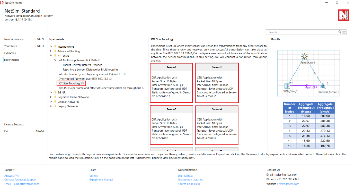
Figure 22‑1: List of scenarios for the example of IOT Star Topology
The simulation scenario consists of n nodes distributed uniformly around a sink (PAN coordinator) at the center. In NetSim the nodes associate with the PAN coordinator at the start of the simulation. CBR traffic is initiated simultaneously from all the nodes. The CBR packet size is kept as 10 bytes to which 20 bytes of IP header, 7 bytes of MAC header and 6 bytes of PHY header are added. To ensure saturation, the CBR traffic interval is kept very small; each node's buffer receives packets at intervals of 5 ms.
Procedure#
Sensor-1
NetSim UI displays the configuration file corresponding to this experiment as shown below Figure 22‑2.

Figure 22‑2: Network set up for studying the Sensor 1
The following set of procedures were done to generate this sample:
Step 1: A network scenario is designed in NetSim GUI comprising of 1 SinkNode, and 1 wireless sensor in the "WSN" Network Library. Distance between the SinkNode and Wireless Sensor is set to 8m.
Step 2: Right click on Adhoc link and select Properties, Channel Characteristics is set to No_Pathloss
Step 3: Right click on Wireless sensor properties in the network layer the static route is configured as shown below Table 22‑1.
+-------------+-----------+-----------------+----------+-------------+ | Network | Gateway | SubnetMask | Metrics | Interface | | | | | | ID | | Destination | | | | | +=============+===========+=================+==========+=============+ | 11.1.1.0 | 11.1.1.1 | 255.255.255.0 | 1 | 1 | +-------------+-----------+-----------------+----------+-------------+
Table 22‑1: Static route for Wireless sensor
Step 4: Right click on the Application Flow App1 CBR and select Properties or click on the Application icon present in the top ribbon/toolbar.
A CBR Application is generated from Wireless Sensor 2 i.e., Source to Sink Node 1 i.e., Destination with Packet Size remaining 10Bytes and Inter Arrival Time remaining 5000µs. Start time is set to 5s.
Transport Protocol is set to UDP instead of TCP.
Step 5: Plots is enabled in NetSim GUI. Click on Run simulation. The simulation time is set to 100 seconds.
Increase wireless sensor count to 2, 3, and 4 with the same above properties to design Sensor- 2, 3, and 4.
Sensor-5: NetSim UI displays the configuration file corresponding to this experiment as shown below Figure 22‑3.

Figure 22‑3: Network set up for studying the Sensor-5
The following set of procedures were done to generate this sample:
Step 1: Right click on Wireless sensors properties in the network layer the static route is configured as shown below Table 22‑2 .
Network Gateway SubnetMask Metrics Interface ID Destination
11.1.1.0 11.1.1.1 255.255.255.0 1 1
Table 22‑2: Static route for Wireless sensors
Step 2: Click on the Application icon present in the top ribbon/toolbar. The following application properties is set shown in below Table 22‑3.
App 1 App 2 App 3 App 4 App 5
Application CBR CBR CBR CBR CBR
Source ID 2 3 4 5 6
Destination ID 1 1 1 1 1
Start time 5s 5s 5s 5s 5s
Transport protocol UDP UDP UDP UDP UDP
Packet Size 10bytes 10bytes 10bytes 10bytes 10bytes
Inter-Arrival Time 5000 μs 5000 μs 5000 μs 5000 μs 5000 μs
Table 22‑3: Detailed Application properties
Step 5: Plots is enabled in NetSim GUI. Click on Run simulation. The simulation time is set to 100 seconds.
Increase wireless sensor count to 10, 15, 20, 25, 30, 35, 40, and 45 with the same above properties to design Sensor-6, 7, 8, 9, 10, 11, 12, and 13.
Output#
The aggregate throughput of the system can be got by adding up the individual throughput of the applications. NetSim outputs the results in units of kilobits per second (kbps). Since the packet size is $80\ bits$ we convert per the formula
$$Aggregate\ Throughput\ (pkts\ per\ sec) = \frac{Aggregate\ Throughput\ (kbps)*1000}{80}$$
Number of Nodes Aggregate Throughput Aggregate Throughput (Kbps) (pkts/s)
1 16.00 200.00
2 23.07 288.38
3 22.67 283.38
4 22.33 279.13
5 21.85 273.13
10 18.60 232.50
15 15.26 190.75
20 12.32 154.00
25 9.98 124.75
30 7.84 98.00
35 6.17 77.13
40 4.88 61.00
45 3.72 46.50
Table 22‑4: Aggregate throughput for Star topology scenario
Figure 22‑4: Plot of Aggregated throughput (packets/s) vs Number of Nodes
Discussion#
In Figure 22‑4 we plot the throughput in packets per second versus the number of IoT devices in the star topology network. We make the following observations:
-
Notice that the throughput for a single saturated node is 200 packets per second, which is just the single hop throughput from a single saturated node, when the packet payload is 10 bytes. When a node is by itself, even though there is no contention, still the node goes through a backoff after every transmission. This backoff is a waste and ends up lowering the throughput as compared to if the node knew it was the only one in the network and sent packets back-to-back.
-
When there are two nodes, the total throughput increases to 287.5 packets per second. This might look anomalous. In a contention network, how can the throughput increase with more nodes? The reason can be found in the discussion of the previous observation. Adding another node helps fill up the time wasted due to redundant backoffs, thereby increasing throughput.
-
Adding yet another node results in the throughput dropping to 282.5 packets per second, as the advantage gained with 2 nodes (as compared to 1 node) is lost due to more collisions.
-
From there on as the number of nodes increases the throughput drops rapidly to about 100 packets per second for about 30 nodes.
-
The above behaviour must be compared with Experiment 12 where several IEEE 802.11 STAs, with saturated queues, were transmitting packets to an AP. The throughput increased from 1 STA to 2 STAs, dropped a little as the number of STAs increased and then flattened out. On the other hand, in IEEE 802.15.4 the throughput drops rapidly with increasing number of STAs. Both IEEE 802.11 and IEEE 802.15.4 have CSMA/CA MACs. However, the adaptation in IEEE 802.11 results in rapid reduction in per-node attempt rate, thus limiting the drop in throughput due to high collisions. On the other hand, in IEEE 802.15.4, the per-node attempt rate flattens out as the number of nodes is increased, leading to high collisions, and lower throughput. We note, however, that IoT networks essentially gather measurements from the sensor nodes, and the measurement rates in most applications are quite small.
References#
- Chandramani Kishore Singh, Anurag Kumar. P. M. Ameer (2007). Performance evaluation of an IEEE 802.15.4 sensor network with a star topology. Wireless Network (2008) 14:543--568