Sample configuration files for all networks are available in Examples Menu in NetSim Home Screen. These files provide examples on how NetSim can be used – the parameters that can be changed and the typical effect it has on performance.
IOT Example Simulations#
Energy Model #
Open NetSim, Select Examples->IOT-WSN->Internet of Things->Energy Model then click on the tile in the middle panel to load the example as shown in Figure 4‑1.

Figure 4‑1: List of scenarios for the example of Energy Model
The following network diagram illustrates, what the NetSim UI displays when you open the example configuration file.

Figure 4‑2: Network set up for studying the Energy Model
Settings done in sample network
-
Grid length(m) 100, Side Length(m) 100, Manually via Click and Drop.
-
In LOWPAN_Gateway change BeaconMode Enable, Superframe Order 10, Beacon Order 10.
-
Channel Characteristic NO PATHLOSS in Adhoc link Properties.

Figure 4‑3: Datalink layer Properties for Lowpan Gateway
-
Click on the Application icon present in the top ribbon/toolbar
- Created Sensor Application from Sensor_1 to Wired_Node_4 with > default Properties.
-
In NetSim GUI Plots are Enabled.
-
Run the simulate for 100 sec.
-
Check the Battery model in simulation results window, users should get zero value for Sleep energy (mJ) consumed.
-
Go back to Simulation window change following properties in LOWPAN_Gateway for another sample.
-
Set Superframe Order (SO) and Beacon Order (BO) as 10 and 12 respectively (0 \<= SO \<= BO \<= 14)
-
Re-run the Simulate for 100 sec.
-
Check the Battery Model metrics in metrics window, users should get non-zero value for Sleep energy consumed.
Results: In Superframe order 10 and Beacon order 10 Sample, users can observe sleep energy consumed value will be zero in Battery Model metrics in the Results Window since sensor is in active state all the time. i.e., if SO=10 and BO=10, there won’t be any inactive portion of the Superframe.

Figure 4‑4: Battery Model Table for SO=10 & BO=10
In Superframe order 10 and Beacon order 12 Sample, sleep energy consumed will be non-zero since sensor goes to sleep mode during the inactive portion of the Superframe.

Figure 4‑5: Battery Model Table for SO=10 & BO=12
Working of RPL Protocol in IoT #
Open NetSim, Select Examples->IOT-WSN->Internet of Things->Working of RPL Protocol in IoT then click on the tile in the middle panel to load the example as shown in Figure 4‑4.

Figure 4‑6: List of scenarios for the example of Working of RPL Protocol in IoT
The following network diagram illustrates, what the NetSim UI displays when you open the example configuration file.

Figure 4‑7: Network set up for studying the Working of RPL Protocol in IoT
Settings done in sample network:
-
Grid length(m) 100m, Side Length(m) 50, Manually via Click and Drop.
-
Routing protocol has set as RPL for 6LOWPAN Gateway and Sensor. Go to properties Network Layer Routing Protocol as shown Figure 4‑6.
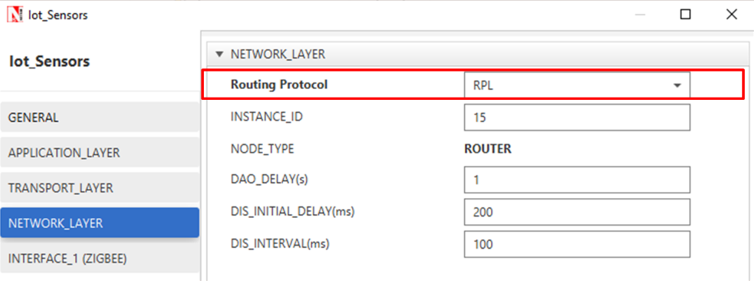
Figure 4‑8: Routing Protocol to RPL in Network layer
-
In Adhoc Link Properties change Channel characteristics Path Loss only, Path Loss Model Log Distance and path loss exponent 3.5
-
Application properties has set as shown in below Table 4‑1.
| Application Properties | |||
|---|---|---|---|
| Application ID | Application Type | Source Id | Destination Id |
| 1 | SENSOR_APP | 1 | 8 |
| 2 | SENSOR_APP | 3 | 8 |
| 3 | SENSOR_APP | 5 | 8 |
Table 4‑1: Application properties
Procedure to get detailed RPL log file:
-
Go to NetSim Home page and click on Your work.
-
Click on Source code and then click on Open Code and open > the codes in Visual Studio. Set x64 according to the NetSim > build which you are using.
-
Go to the RPL Project in the Solution Explorer. Open RPL.h file and > change //#define DEBUG_RPL to #define DEBUG_RPL as shown > below Figure 4‑7.

Figure 4‑9: Visual Studio
-
Right click on the RPL project in the solution explorer and > click on rebuild.
-
After the RPL project is rebuild successful, go back to the network > scenario.
-
In NetSim GUI Plots are Enabled. Run simulation for 100 sec and go > to Result window Log Files, open rpl log file.

Figure 4‑10: Simulation Result window
Results

Figure 4‑11: RPL log file
The observations of rpl log file which is generated in NetSim is given in the below Table 4‑2.
| Node | Rank | Updated Rank | Parent list | Updated Parent Node ID | Sibling Node ID | Received DIO From Node ID |
|---|---|---|---|---|---|---|
| Node 1 | 30 | 28 | Node 2, Node 4 | Node 2 | Node 3 | Node 2, Node 3, Node 4 |
| Node 2 | 15 | 15 | Node 6 | Node 6 | Node 4 | Node 4, Node 6 |
| Node 3 | 28 | 28 | Node 2, Node 4, Node 5 | Node 4 | Node 1 | Node 1, Node 2, Node 4, Node 5 |
| Node 4 | 15 | 15 | Node 6 | Node 6 | Node 2 | Node 2, Node 6 |
| Node 5 | 27 | 27 | Node 4 | Node 4 | - | Node 4 |
Table 4‑2: RPL Log file contains Rank, Updated Rank, parent list, Updated Parent Node ID, Sibling Node ID and Received DIO From Node ID etc.
The above table can be summarized as follows:
DIO message is sent by the root node, i.e. LowPAN Gateway, with Rank 1 to Sensor 2 and Sensor 4 as shown Figure 4‑10.

Figure 4‑12: DIO messages sent by the LOWPAN Gateway to Sensors
On receiving the DIO message, Node 4 will recognize the DODAG Id of Root Node and identifies it as Parent node. Rank of Node 4 will get updated to 15. Also, Node 2 is recognized as sibling of Node 4.
Now, node 4 will broadcast DIO message to other nodes as shown Figure 4‑11.

Figure 4‑13: Wireless Sensor 4 broadcasting DIO message to other Sensors
Node 1 receives DIO message from Node 4 and it identifies the DODAG Id of Node 4. Hence, Node 1 recognizes Node 4 as the Parent Node. Rank of Node 1 will get updated to 30. As Node 3 is within the range of Node1, Node 3 is identified as a sibling of Node1.
Node 1 will then broadcast DIO messages as shown Figure 4‑12.

Figure 4‑14: Wireless Sensor 1 broadcasting DIO message to other Sensors
Node 2 receives the DIO message from Node 6 and identifies it as Parent node. The Rank of Node 2 gets updated to 15. Node 2 now broadcasts the DIO message to other nodes as shown Figure 4‑13.

Figure 4‑15: Wireless Sensor 2 broadcasting DIO message to other Sensors
Node 3 receives DIO message from Node 2 and the rank of Node 3 gets updated to 28. Node 2 is identified as the parent node of Node 3.
Node 3 then broadcasts DIO message to other nodes as shown Figure 4‑14.

Figure 4‑16: Wireless Sensor 3 broadcasting DIO message to other Sensors
Node 5 receives DIO message from Node 3, hence, it identifies Node 4 as th parent node. The rank of Node 5 gets updated to 27.
Node 5 then broadcasts DIO message as shown Figure 4‑15.

Figure 4‑17: Wireless Sensor 5 broadcasting DIO message to other Sensors
Further, Node 1 receives DIO message from Node 2 and the parent list of Node 1 gets updated to Node 4 and Node 2. Also, the rank of Node 1 gets updated to 28.
According to the link quality, DODAG is formed.
-
Node 2 and Node 4 are siblings and their parent is Node 6 (Root > Node). Rank is 15.
-
Node 1 and Node 3 are siblings.
-
Node 1 established its parent as Node 2. Rank is 28.
-
Node 3 establishes its parent as Node 4. Rank is 28.
-
-
Node 5 doesn’t have any siblings and establishes its parent as > Node 4. Its rank is 27.

Figure 4‑18: Based on link quality, DODAG is formed and Rank assigned to sensors and lowpan gateway
Modes of Operation in IoT RPL #
The DODAG nodes process the DAO messages according to the RPL Mode of Operations (MOP), which are presented below. Independent of the MOP used, DAO messages may require reception confirmation, which should be done using DAO-ACK messages.
Although it is designed for the Multipoint-to-Point (MP2P) traffic pattern, RPL also admits the data forwarding using Point-to-Multipoint (P2MP) and Point-to-Point (P2P). In MP2P, the nodes send data messages to the root, creating an upward flow as shown in Figure 4‑17: Multipoint to Point. In P2MP, sometimes termed as multicast, the root sends data messages to the other nodes, producing a downward flow depicted in Figure 4‑18: Point to Multipoint..
In P2P, a node sends messages to the other node (non-root) of DODAG; thus, both upward and downward forwarding may be required as illustrated in Figure 4‑19: Point to Point. RPL defines four MOPs that should be used considering the traffic pattern required by the application and the computational capacity of the nodes. In the first, MOP 0 (Point to multipoint), RPL does not maintain downward routes; thus, consequently, only MP2P traffic is enabled. In non-storing MOP (MOP 1 (Multipoint to point)), downward routes are supported, and the use of P2P and MP2P is allowed. However, all downward routes are maintained in the root node. Thus, the total downward traffic should be initially sent to the DODAG root and subsequently be forwarded to its destination as shown in Figure 4‑20: RPL Non-Storing Mode. In storing without multicast MOP (MOP 2 (Point to point)), downward routes are also supported, but are different from MOP 1; the nodes maintain, individually, a routing table constructed using DAO messages to provide downward traffic. Hence, downward forwarding occurs without the use of the root node, as illustrated in Figure 4‑21: RPL Storing Mode. Storing with multicast MOP (MOP 3 (non-Storing mode)) has a functioning similar to MOP 2 (Point to point) plus the possibility of multicast data sending. This type of transmission permits the non-root node to send messages to a group of nodes formed using multicast DAOs.
Figure 4‑19: Multipoint to Point |
Figure 4‑20: Point to Multipoint |
Figure 4‑21: Point to Point |
|
|---|---|---|---|
Figure 4‑22: RPL Non-Storing Mode |
Figure 4‑23: RPL Storing Mode |
||


Open NetSim, Select Examples->IOT-WSN->Internet of Things->Mode of Operations IoT RPL then click on the tile in the middle panel to load the example as shown in Figure 4‑22.
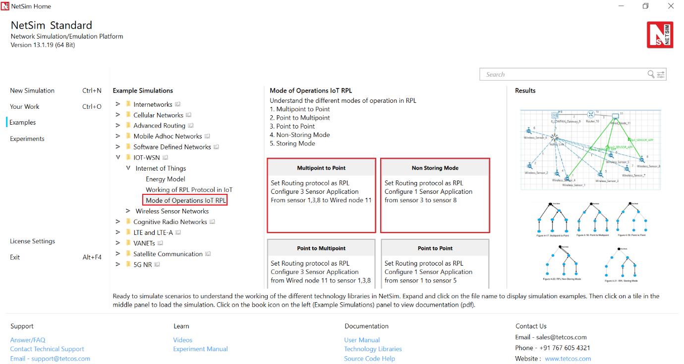
Figure 4‑24: List of scenarios for the example of Mode of Operations IoT RPL
The following network diagram illustrates, what the NetSim UI displays when you open the example configuration file.

Figure 4‑25: Network set up for studying the Mode of Operations IoT RPL
Multipoint to Point#
Settings done in sample network
-
Grid length(m) 100m, manually via Click and Drop.
-
Routing protocol has set as RPL for 6LOWPAN Gateway and Sensor. Go to properties Network Layer Routing Protocol as shown Figure 4‑24.

Figure 4‑26: Routing Protocol to RPL in Network layer
-
In Adhoc Link Properties change Channel characteristics Path Loss only, Path Loss Model Log Distance and path loss exponent 4.2.
-
Application properties has set as shown in below Table 4‑3.
| Application Properties | |||
|---|---|---|---|
| Application ID | Application Type | Source Id | Destination Id |
| 1 | SENSOR_APP | 1 | 11 |
| 2 | SENSOR_APP | 3 | 11 |
| 3 | SENSOR_APP | 8 | 11 |
Table 4‑3: Application properties
-
In NetSim GUI Plots and Packet Traces are Enabled. Run simulation 100s and observe that all the sensors are sending data to route node in animation window and also in packet trace.
Result
Animation window: The nodes send data messages to the root, creating an upward flow,

Figure 4‑27: Animation window for Multipoint to Point
Packet trace: Once the simulation is completed, to view the packet trace file, click on “Open Packet Trace” option present in the left-hand-side of the Results Dashboard and filter the PACKET_TYPE to Sensing. you can observe the flow of Sensor Application packets as shown below:

Figure 4‑28: Packet Trace for Multipoint to Point
Point to Multipoint#
Settings done in sample network
-
Set the all the properties same as Multipoint to Point scenario
-
Application properties has set as shown in below Table 4‑4.
| Application Properties | |||
|---|---|---|---|
| Application ID | Application Type | Source Id | Destination Id |
| 1 | SENSOR_APP | 11 | 1 |
| 2 | SENSOR_APP | 11 | 3 |
| 3 | SENSOR_APP | 11 | 8 |
Table 4‑4: Application properties
-
In NetSim GUI Plots are Enabled. Run simulation 100s and observe that all the sensors are sending data to route node in animation window and also in packet trace.
Result
Animation window: Root sends data messages to the other nodes, producing a downward flow.

Figure 4‑29: Animation window for Point to Multipoint
Packet trace: Once the simulation is completed, to view the packet trace file, click on “Open Packet Trace” option present in the left-hand-side of the Results Dashboard and filter the PACKET_TYPE to Sensing, you can observe the flow of Sensor Application packets as shown below:

Figure 4‑30: Packet trace for Point to Multipoint
Point to Point#
Settings done in sample network
-
Set the all the properties same as Multipoint to Point scenario.
-
Application properties has set as shown in below Table 4‑5.
| Application Properties | |||
|---|---|---|---|
| Application ID | Application Type | Source Id | Destination Id |
| 1 | SENSOR_APP | 1 | 5 |
Table 4‑5: Application properties
-
In NetSim GUI Plots are Enabled. Run simulation 100s and observe that all the sensors are sending data to route node in animation window and also in packet trace.
Result
Animation window: Root sends data messages to the other nodes, producing a downward flow.

Figure 4‑31: Animation window for Point to Point
Packet trace: Once the simulation is completed, to view the packet trace file, click on “Open Packet Trace” option present in the left-hand-side of the Results Dashboard and filter the PACKET_TYPE to Sensing, you can observe the flow of Sensor Application packets as shown below:

Figure 4‑32: Packet trace for Point to Point
Non-storing Mode#
Settings done in sample network
-
Set the all the properties same as Multipoint to Point scenario.
-
Application properties has set as shown in below table:
| Application Properties | |||
|---|---|---|---|
| Application ID | Application Type | Source Id | Destination Id |
| 1 | SENSOR_APP | 3 | 8 |
Table 4‑6: Application properties
-
In NetSim GUI Plots are Enabled. Run simulation 100s and observe > that all the sensors are sending data to route node in animation > window and also in packet trace.
Result
Animation window: In non-storing MOP (MOP 1 (Point to Multipoint)), downward routes are supported, and the use of P2P and MP2P is allowed. However, all downward routes are maintained in the root node. Thus, the total downward traffic should be initially sent to the DODAG root and subsequently be forwarded to its destination.

Figure 4‑33: Animation window for RPL Non-Storing Mode
Packet trace: Once the simulation is completed, to view the packet trace file, click on “Open Packet Trace” option present in the left-hand-side of the Results Dashboard and filter the PACKET_TYPE to Sensing, you can observe the flow of Sensor Application packets as shown below:

Figure 4‑34: Packet trace for RPL Non-Storing Mode
Storing Mode#
Settings done in sample network
-
Set the all the properties same as Multipoint to Point scenario
-
Application properties has set as shown in below Table 4‑7.
| Application Properties | |||
|---|---|---|---|
| Application ID | Application Type | Source Id | Destination Id |
| 1 | SENSOR_APP | 3 | 8 |
Table 4‑7: Application properties
-
In NetSim GUI Plots are Enabled. Run simulation 100s and observe that all the sensors are sending data to root node in animation window and also in packet trace.
Result
Animation window: In storing without multicast MOP (MOP 2 (Point to point)), downward routes are also supported, but are different from MOP 1 (Point to multipoint); the nodes maintain, individually, a routing table constructed using DAO messages to provide downward traffic. Hence, downward forwarding occurs without the use of the root node

Figure 4‑35: Animation window for RPL Storing Mode
Packet trace: Once the simulation is completed, to view the packet trace file, click on “Open Packet Trace” option present in the left-hand-side of the Results Dashboard and filter the PACKET_TYPE to Sensing, you can observe the flow of Sensor Application packets as shown below.

Figure 4‑36: Packet trace for RPL Storing Mode
WSN Example Simulation#
Beacon Time Analysis #
Open NetSim, Select Examples->IOT-WSN->Wireless Sensor Networks->Beacon Time Analysis then click on the tile in the middle panel to load the example as shown in Figure 4‑35.

Figure 4‑37: List of scenarios for the example of Beacon Time Analysis
The following network diagram illustrates, what the NetSim UI displays when you open the example configuration file.

Figure 4‑38: Network set up for studying the Beacon Time Analysis
Settings done in sample config file
-
The following Environment properties are already set, as Manually Via Click and Drop.
-
In SinkNode->INTERFACE_1(Zigbee)> Datalink Layer enable Beacon mode set Superframe Order (SO) -> 10 and Beacon Order (BO) -> 12

Figure 4‑39: Datalink layer Properties window for Sink node
-
In Adhoc Link Properties change Channel characteristics-> Path Loss only, Path Loss Model -> Log Distance and path loss exponent ->2.
-
Generate SENSOR_APP Traffic Between Wireless_Sensor_1 to WSN_Sink_3 and set the transport layer protocol as UDP and other properties are default.
-
Enable Packet Trace and Plots.
-
Set Simulation time as 200 sec.
Theoretical Beacon Time Calculation
-
Beacon Interval (BI)= Super Frame duration (Active Period) + > Inactive Period (IP).
-
$BI\ = \ abasesuperframe\ duration \times 2\ \hat{}BO\ = \ 15.36ms\ \times \ 2\hat{}12\ = \ 62914.56ms\ \sim\ 62s.$
-
$SD\ = \ abasesuperframe\ duration \times 2\ \hat{}SO\ = \ 15.36ms\ \times 2\hat{}10\ = \ 15728.64ms.$
-
To find Inactive period, IP = BI – SD = 62914.56ms - 15728.64ms = > 47185.92ms.
-
Super Frame duration is divided into 16 slots (1st slot > is allocated for beacon frame).
-
Each slot time = 15728.64ms / 16 = 983.04ms
NetSim Results:
- Open packet trace and filter CONTROL_PACKET_TYPE to > Zigbee_BEACON_FRAME, users should get four zigbee_beacon_frames at > 0, 62.9, 125.8, 188.7 secs (approx.) for each Sensor_Node, because > the time interval between two beacons frames is 62 seconds. Since > we have 2 nodes so user can get 4 beacon frames for each node.

Figure 4‑40: Packet Trace Window of Beacon Time Analysis
- 4 beacons were transmitted, so > beacon time = 983.04ms× 4 = 3932.16millisec (since > 1 beacon = 1 time slot). Check the beacon time in IEEE 802.15.4 > metrics window.
CAP Time Analysis #
Open NetSim, Select Examples->IOT-WSN->Wireless Sensor Networks->CAP Time Analysis then click on the tile in the middle panel to load the example as shown in Figure 4‑38.

Figure 4‑41: List of scenarios for the example of CAP Time Analysis
The following network diagram illustrates, what the NetSim UI displays when you open the example configuration file.

Figure 4‑42: Network set up for studying the CAP Time Analysis
Settings done in example config file
-
The following Environment properties are already set, as Manually Via Click and Drop.
-
In SinkNode->INTERFACE_1(Zigbee)> Datalink Layer enable Beacon mode set Superframe Order (SO) -> 10 and Beacon Order (BO) -> 12
Figure 4‑43: Datalink layer Properties window for Sink node
-
In Adhoc Link Properties change Channel characteristics -> Path Loss only, Path Loss Model -> Log Distance and path loss exponent -> 2.
-
Generate SENSOR_APP Traffic Between Wireless_Sensor_1 to WSN_Sink_3 and set the transport layer protocol as UDP other properties are default.
-
Enable Packet Trace and Plots.
-
Set Simulation time as 100 sec.
Theoretical CAP Time Calculation
-
To find CAP time, BI is 62914.56ms -> So in 100s, two beacon frames should be transmitted at 0 & 62s.
-
Check no. of beacon frames transmitted in 802.15.4 metrics.
-
Here CFP = 0 because there is only 1 sensor.
-
CAP Time = SD – beacon time = (15728.64ms) – (983.04ms) = 14745.6ms.
-
Open packet trace and filter Control_Packet_Type to Zigbee_Beacon_Frame, users should get two zigbee_beacon_frames at 0, 62.9secs, because the time interval between two beacon frames is 62 seconds. Since we have 2 nodes so user can get 2 beacon frames for each node.
-
Since two Beacon frames are transmitted,
CAP time = 2× 14745.6ms = 29491200µs.
NetSim Results:
-
Check and compare the theoretical CAP time with NetSim simulation results in IEEE 802.15.4 metrics in Results Windows.
-
CAP time = 29491200.0000Microsec.

Figure 4‑44: IEEE802.15.4_Metrics_Table in Results Windows
Static Routing in WSN #
Open NetSim, Select Examples->IOT-WSN->Wireless Sensor Networks->WSN Static Route then click on the tile in the middle panel to load the example as shown in Figure 4‑41.

Figure 4‑45: List of scenarios for the example of WSN Static Route
The following network diagram illustrates, what the NetSim UI displays when you open the example configuration file.

Figure 4‑46: Network set up for studying the WSN Static Route
Without Static Route
Settings done in the network
-
The following Environment properties are already set, as Manually > Via Click and Drop.
-
Set Application type as SENSOR_APP Source_Id as 1 and Destination_Id > as 6
-
Enable Packet trace and Plot option.
-
Click on run simulation and set Simulation Time as 100 sec.
Results: Open packet animation and check Sensor 1 would send packets directly to the destination.
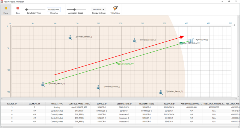
Figure 4‑47: Packet animation window
Open packet trace and filter PACKET_TYPE column as Sensing and observe the packets flow.

Figure 4‑48: Packet Trace
With Static Route
Settings done in the network
- In Without Static Route, we have changed Wireless_Sensor > properties as per the following.
Configuring Static Routes
Open Wireless_Sensor properties, go to network layer and Enable - Static IP Route ->click on Configure Static Route IP link, set Network Destination, Gateway, Subnet Mask, Metrics, and Interface ID as shown in below screenshot and click on ADD.

Figure 4‑49: Static IP Routing Configuring window
| Device | Network Destination | Gateway | Subnet Mask | Metrics | Interface ID |
|---|---|---|---|---|---|
| Wireless_Sensor_1 | 11.1.0.0 | 11.1.1.3 | 255.255.0.0 | 1 | 1 |
| Wireless_Sensor_2 | 11.1.0.0 | 11.1.1.4 | 255.255.0.0 | 1 | 1 |
| Wireless_Sensor_3 | 11.1.0.0 | 11.1.1.5 | 255.255.0.0 | 1 | 1 |
| Wireless_Sensor_4 | 11.1.0.0 | 11.1.1.6 | 255.255.0.0 | 1 | 1 |
Table 4‑8: Static Route Configuration for Sensors
-
After setting the properties click on run simulation and set > Simulation Time as 100 sec.
Results
Open packet animation and check packets would reach the destination via the configured static route,
SENSOR_1 SENSOR_2 SENSOR_3 SENSOR_4 SENSOR_5 SINKNODE_6

Figure 4‑50: Packets flow in animation window as specified in the static route configuration
Open packet trace and filter PACKET_TYPE column to Sensing and observe the packets flow as specified in the static route configuration.
SENSOR_1 SENSOR_2 SENSOR_3 SENSOR_4 SENSOR_5 SINKNODE_6

Figure 4‑51: Packet flow in Packet Trace