Introduction#
Delay is another important measure of quality of a network, very relevant for real-time applications. The application processes concern over different types of delay - connection establishment delay, session response delay, end-to-end packet delay, jitter, etc. In this experiment, we will review the most basic and fundamental measure of delay, known as end-to-end packet delay in the network. The end-to-end packet delay denotes the sojourn time of a packet in the network and is computed as follows. Let $a_{i}\ $and $d_{i}\ $ denote the time of arrival of packet $i$ into the network (into the transport layer at the source node) and time of departure of the packet $i$ from the network (from the transport layer at the destination node), respectively. Then, the sojourn time of the packet i is computed as ($d_{i} - a_{i}$ ) seconds. A useful measure of delay of a flow is the average end-to-end delay of all the packets in the flow, and is computed as
$$average\ packet\ delay = \frac{1}{N}\sum_{i = 1}^{N}\left( d_{i - \ }a_{i}^{\ } \right)secs\ $$
where, N is the count of packets in the flow.
A packet may encounter delay at different layers (and nodes) in the network. The transport layer at the end hosts may delay packets to control flow rate and congestion in the network. At the network layer (at the end hosts and at the intermediate routers), the packets may be delayed due to queues in the buffers. In every link (along the route), the packets see channel access delay and switching/forwarding delay at the data link layer, and packet transmission delay and propagation delay at the physical layer. In addition, the packets may encounter processing delay (due to hardware restrictions). It is a common practice to group the various components of the delay under the following four categories: queueing delay (caused due to congestion in the network), transmission delay (caused due to channel access and transmission over the channel), propagation delay and processing delay. We will assume zero processing delay and define packet delay as
$$end\ to\ end\ packet\ delay\ = queueing\ delay + transmission\ delay\ + \ propagation\ delay$$
We would like to note that, in many scenarios, the propagation delay and transmission delay are relatively constant in comparison with the queueing delay. This permits us (including applications and algorithms) to use packet delay to estimate congestion (indicated by the queueing delay) in the network.
Little's Law#
The average end-to-end packet delay in the network is related to the average number of packets in the network. Little's law states that the average number of packets in the network is equal to the average arrival rate of packets into the network multiplied by the average end-to-end delay in the network, i.e.,
$$average\ number\ of\ packets\ in\ the\ network = average\ arrival\ rate\ into\ the\ network \times$$
$$\ \ \ \ \ \ \ \ \ \ \ \ \ \ \ \ \ \ \ \ \ \ \ \ \ \ \ \ \ \ \ \ \ \ \ \ \ \ \ \ \ \ \ \ \ \ \ \ \ \ \ \ \ \ \ \ \ \ \ \ \ \ \ \ \ \ \ \ \ \ \ \ \ \ \ \ \ \ \ \ \ \ \ \ \ \ \ average\ end\ to\ end\ delay\ in\ the\ network$$
Likewise, the average queueing delay in a buffer is also related to the average number of packets in the queue via Little's law.
$$average\ number\ of\ packets\ in\ queue = average\ arrival\ rate\ into\ the\ queue \times$$
$$\ \ \ \ \ \ \ \ \ \ \ \ \ \ \ \ \ \ \ \ \ \ \ \ \ \ \ \ \ \ \ \ \ \ \ \ \ \ \ \ \ \ \ \ \ \ \ \ \ \ \ \ \ \ \ \ \ \ \ \ \ \ \ \ \ \ \ \ \ \ \ \ \ \ \ \ average\ delay\ in\ the\ queue$$
The following figure illustrates the basic idea behind Little's law. In Figure 4‑1a, we plot the arrival process $a(t)$ (thick black line) and the departure process $d(t)$ (thick red line) of a queue as a function of time. We have also indicated the time of arrivals $(a_{i})$ and time of departures $(d_{i})$ of the four packets in Figure 4‑1a. In Figure 4‑1b, we plot the queue process $q(t) = a(t) - d(t)$ as a function of time, and in Figure 4‑1c, we plot the waiting time $\left( d_{i - \ }a_{i}^{\ } \right)$ of the four packets in the network. From the figures, we can note that the area under the queue process is the same as the sum of the waiting time of the four packets. Now, the average number of packets in the queue ( $\frac{14}{10}$ , if we consider a duration of ten seconds for the experiment) is equal to the product of the average arrival rate of packets $\left( \frac{4}{10} \right)$ and the average delay in the queue $\left( \frac{14}{4} \right)$.

Figure 4‑1: Illustration of Little's law in a queue
In Experiment 3 (Throughput and Bottleneck Server Analysis), we noted that bottleneck server analysis can provide tremendous insights on the flow and network performance. Using M/G/1 analysis of the bottleneck server and Little's law, we can analyze queueing delay at the bottleneck server and predict end-to-end packet delay as well (assuming constant transmission times and propagation delays).
NetSim Simulation Setup#
Open NetSim and click on Experiments> Internetworks> Network Performance> Delay and Littles Law then click on the tile in the middle panel to load the example as shown in below screenshot
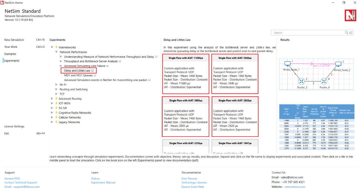
Figure 4‑2: List of scenarios for the example of Delay and Littles Law
Part-1: A Single Flow Scenario#
We will study a simple network setup with a single flow illustrated in Figure 4‑3 to review end to end packet delay in a network as a function of network traffic. An application process at Wired Node 1 seeks to transfer data to an application process at Wired_Node_2. We will consider a custom traffic generation process (at the application) that generates data packets of constant length (say, L bits) with i.i.d. inter-arrival times (say, with average inter-arrival time $v$ seconds). The application traffic generation rate in this setup is $\frac{L}{v}$ bits per second. We prefer to minimize communication overheads (including delay at the transport layer) and hence, will use UDP for data transfer between the application processes.
In this setup, we will vary the traffic generation rate $\left( \frac{L}{v} \right)$ by varying the average inter-arrival time $(v)$, and review the average queue at the different links, average queueing delay at the different links and end-to-end packet delay.
Procedure#
We will simulate the network setup illustrated in Figure 4‑3 with the configuration parameters listed in detail in Table 4‑1 to study the single flow scenario.
NetSim UI displays the configuration file corresponding to this experiment as shown below:

Figure 4‑3: Network set up for studying a single flow
The following set of procedures were done to generate this sample:
Step 1: Drop two wired nodes and two routers onto the simulation environment. The wired nodes and the routers are connected with wired links as shown in (See Figure 4‑3).
Step 2: Click the Application icon to configure a custom application between the two wired nodes. In the Application configuration dialog box (see Figure 4‑4), select Application Type as CUSTOM, Source ID as 1 (to indicate Wired_Node_1), Destination ID as 2 (to indicate Wired_Node_2) and Transport Protocol as UDP. In the PACKET SIZE tab, select Distribution as CONSTANT and Value as 1460 bytes. In the INTER ARRIVAL TIME tab, select Distribution as EXPONENTIAL and Mean as 11680 microseconds.

Figure 4‑4: Application configuration dialog box
Step 3: The properties of the wired nodes are left to the default values.
Step 4: Right-click the link ID (of a wired link) and select Properties to access the link's properties dialog box (see Figure 4‑5). Set Max Uplink Speed and Max Downlink Speed to 10 Mbps for link 2 (the backbone link connecting the routers) and 1000 Mbps for links 1 and 3 (the access link connecting the Wired_Nodes and the routers). Set Uplink BER and Downlink BER as 0 for links 1, 2 and 3. Set Uplink_Propagation_Delay and Downlink_Propagation_
Delay as 0 microseconds for the two-access links 1 and 3 and 10 milliseconds for the backbone link 2.

Figure 4‑5: Link Properties dialog box
Step 5: Right-click Router 3 icon and select Properties to access the link's properties dialog box (see Figure 4‑6). In the INTERFACE 2 (WAN) tab, select the NETWORK LAYER properties, set Buffer size (MB) to 8.

Figure 4‑6: Router Properties dialog box
Step 6: Click on Packet Trace option and select the Enable Packet Trace check box. Packet Trace can be used for packet level analysis.
Step 7: Click on Run icon to access the Run Simulation dialog box (see Figure 4‑7) and set the Simulation Time to 100 seconds in the Simulation Configuration tab. Now, run the simulation.

Figure 4‑7: Run Simulation dialog box
Step 8: Now, repeat the simulation with different average inter-arrival times (such as 5840 µs, 3893 µs, 2920 µs, 2336 µs and so on). We vary the input flow rate by varying the average inter-arrival time. This should permit us to identify the bottleneck link and the maximum achievable throughput.
The detailed list of network configuration parameters are presented in (See Table 4‑1).
| Parameter | Value |
|---|---|
| LINK PARAMETERS | |
| Wired Link Speed (access link) | 1000 Mbps |
| Wired Link Speed (backbone link) | 10 Mbps |
| Wired Link BER | 0 |
| Wired Link Propagation Delay (access link) | 0 |
| Wired Link Propagation Delay (backbone link) | 10 milliseconds |
| APPLICATION PARAMETERS | |
| Application | Custom |
| Source ID | 1 |
| Destination ID | 2 |
| Transport Protocol | UDP |
| Packet Size – Value | 1460 bytes |
| Packet Size - Distribution | Constant |
| Inter Arrival Time – Mean | AIAT (µs) Table 4 2 |
Inter Arrival Time - Distribution | Exponential ROUTER PARAMETERS Buffer Size | 8 MISCELLANEOUS Simulation Time | 100 Sec Packet Trace | Enabled Plots | Enabled
Table 4‑1: Detailed Network Parameters
Performance Measure#
In Table 4‑2 and Table 4‑3, we report the flow average inter-arrival time $v$ and the corresponding application traffic generation rate, input flow rate (at the physical layer), average queue and delay of packets in the network and in the buffers, and packet loss rate.
Given the average inter-arrival time $v$ and the application payload size L bits (here, 1460×8 = 11680 bits), we have,
$$Traffic\ generation\ rate = \frac{L}{v} = \frac{11680}{v}bps$$
$$input\ flow\ rate = \frac{11680 + 54 \times 8}{v} = \frac{12112}{v}bps$$
where the packet overheads of 54 bytes is computed as $54 = 8(UDP\ header) + 20(IP\ header) + 26(MAC + PHY\ header)\ bytes$.
Let $Q_{l}(u)$ as denote the instantaneous queue at link $l$ at time $u$ . Then, the average queue at link $l$ is computed as
$$average\ queue\ at\ link\ l = \frac{1}{T}\int_{0}^{T}{Q_{l\ \ }(u)}\ \ du\ bits$$
where, T is the simulation time. And, let $N(u)$ denote the instantaneous number of packets in the network at time $u$. Then, the average number of packets in the network is computed as
$$average\ number\ of\ packet\ in\ the\ network\ = \frac{1}{T}\int_{0}^{T}{N(u)}\ \ du\ bits$$
Let $a_{i,l}$ and $d_{i,l}$ denote the time of arrival of a packet $i$ into the link $l$ (the corresponding router) and the time of departure of the packet $i$ from the link $l$ (the corresponding router), respectively. Then, the average queueing delay at the link $l$ (the corresponding router) is computed as
$$average\ queueing\ delay\ at\ link\ l = \frac{1}{N}\sum_{i = 1}^{N}\left( d_{i,l - \ }a_{i,l}^{\ } \right)$$
where N is the count of packets in the flow. Let ai and di denote the time of arrival of a packet i into the network (into the transport layer at the source node) and time of departure of the packet i from the network (from the transport layer at the destination node), respectively. Then, the end-to-end delay of the packet $i$ is computed as $\left( d_{i - \ }a_{i}^{\ } \right)$ seconds, and the average end to end delay of the packets in the flow is computed as
$$average\ end\ to\ end\ packet\ delay = \frac{1}{N}\sum_{i = 1}^{N}\left( d_{i - \ }a_{i} \right)$$
Average Queue Computation from Packet Trace#
-
Open Packet Trace file using the Open Packet Trace option available in the Simulation Results window.
-
In the Packet Trace, filter the data packets using the column CONTROL PACKET TYPE/APP NAME and the option App1 CUSTOM (see Figure 4‑8).

Figure 4‑8: Filter the data packets in Packet Trace by selecting App1 CUSTOM
-
Now, to compute the average queue in Link 2, we will select TRANSMITTER_ID as ROUTER-3 and RECEIVER_ID as ROUTER-4. This filters all the successful packets from Router 3 to Router 4.
-
The columns NW_LAYER_ARRIVAL_TIME(US) and PHY_LAYER_ARRIVAL TIME(US) correspond to the arrival time and departure time of the packets in the buffer at Link 2, respectively (see Figure 4‑9).
-
You may now count the number of packets arrivals (departures) into (from) the buffer up to time $t$ using the NW_LAYER_ARRIVAL_TIME(US) (PHY_LAYER_ARRIVAL TIME(US)) column. The difference between the number of arrivals and the number of departures gives us the number of packets in the queue at any time.

Figure 4‑9: Packet arrival and departure times in the link buffer
-
Calculate the average queue by taking the mean of the number of packets in queue at every time interval during the simulation.
-
The difference between the PHY LAYER ARRIVAL TIME(US) and the NW LAYER ARRIVAL TIME(US) will give us the delay of a packet in the link (see Figure 4‑10).
$$Queuing\ Delay = \ PHY\ LAYER\ ARRIVAL\ TIME(US)\ –\ NW\ LAYER\ ARRIVAL\ TIME(US)$$

Figure 4‑10: Queuing Delay
- Now, calculate the average queuing delay by taking the mean of the queueing delay of all the packets (see Figure 4‑10)
Network Delay Computation from Packet Trace#
-
Open Packet Trace file using the Open Packet Trace option available in the Simulation Results window
-
In the Packet Trace, filter the data packets using the column CONTROL PACKET TYPE/APP NAME and the option App1 CUSTOM (see Figure 4‑8).
-
Now, we will select the RECEIVER ID as NODE-2. This filters all the successful packets in the network that reached Wired Node 2
-
The columns APP LAYER ARRIVAL TIME(US) and PHY LAYER END TIME(US) correspond to the arrival time and departure time of the packets in the network respectively.
-
You may now count the number of arrivals (departures) into (from) the network upto time t using the APP LAYER ARRIVAL TIME(US) (PHY LAYER END TIME(US)) column. The difference between the number of arrivals and the number of departures gives us the number of packets in the network at any time.
-
Calculate the average number of packets in the network by taking the mean of the number of packets in network at every time interval during the simulation.
-
Packet Delay at a per packet level can be calculated using the columns Application Layer Arrival Time and Physical Layer End Time in the packet trace as:
End-to-End Delay = PHY LAYER END TIME(US) -- APP LAYER ARRIVAL TIME(US)
- Calculate the average end-to-end packet delay by taking the mean of the difference between Phy Layer End Time and App Layer Arrival Time columns
Note: To calculate average number of packets in queue refer the experiment on Throughput and Bottleneck Server Analysis.
Results#
In Table 4‑2, we report the flow average inter-arrival time (AIAT) and the corresponding application traffic generation rate (TGR), input flow rate (at the physical layer), average number of packets in the system, end-to-end packet delay in the network and packet loss rate.
| AIAT v (in µs) | TGR $\frac{L}{v}$ (in Mbps) | Input Flow Rate(in Mbps) | Arrival Rate (in Pkts/sec) | Avg no of packets in system | End-to-End Packet Delay (in µs) | Packet Loss Rate (in percent) |
|---|---|---|---|---|---|---|
| 11680 | 1 | 1.037 | 86 | 0.97 | 11282.188 | 0.01 |
| 5840 | 2 | 2.074 | 171 | 1.94 | 11367.905 | 0.01 |
| 3893 | 3.0003 | 3.1112 | 257 | 2.94 | 11474.118 | 0.01 |
| 2920 | 4 | 4.1479 | 342 | 3.98 | 11621.000 | 0.02 |
| 2336 | 5 | 5.1849 | 428 | 5.06 | 11833.877 | 0.01 |
| 1947 | 5.999 | 6.2209 | 514 | 6.24 | 12142.376 | 0.01 |
| 1669 | 6.9982 | 7.257 | 599 | 7.58 | 12664.759 | 0.01 |
| 1460 | 8 | 8.2959 | 685 | 9.48 | 13846.543 | 0.01 |
| 1298 | 8.9985 | 9.3313 | 770 | 13.73 | 17840.278 | 0.02 |
| 1284 | 9.0966 | 9.433 | 779 | 14.73 | 18917.465 | 0.02 |
| 1270 | 9.1969 | 9.537 | 787 | 15.98 | 20318.735 | 0.02 |
| 1256 | 9.2994 | 9.6433 | 796 | 17.74 | 22299.341 | 0.01 |
| 1243 | 9.3966 | 9.7442 | 805 | 20.31 | 25243.577 | 0.01 |
| 1229 | 9.5037 | 9.8552 | 814 | 25.77 | 31677.196 | 0.03 |
| 1217 | 9.5974 | 9.9523 | 822 | 35.06 | 42660.631 | 0.02 |
| 1204 | 9.701 | 10.0598 | 831 | 51.87 | 62466.981 | 0.06 |
| 1192 | 9.7987 | 10.1611 | 839 | 101.21 | 120958.109 | 0.268 |
| 1180 | 9.8983 | 10.2644 | 847 | 442.71 | 528771.961 | 1.152 |
| 1168 | 10 | 10.3699 | 856 | 856.98 | 1022677.359 | 2.105 |
| 1062 | 10.9981 | 11.4049 | 942 | 3876.87 | 4624821.867 | 11.011 |
| 973 | 12.0041 | 12.4481 | 1028 | 4588.84 | 5479885.160 | 18.541 |
| 898 | 13.0067 | 13.4878 | 1114 | 4859.68 | 5797795.877 | 24.758 |
| 834 | 14.0048 | 14.5228 | 1199 | 4998.91 | 5964568.493 | 30.100 |
| 779 | 14.9936 | 15.5481 | 1284 | 5081.93 | 6066291.390 | 34.756 |
Table 4‑2: Packet arrival rate, average number of packets in the system, end-to-end delay and packet loss rate
Calculation
Calculation done for AIAT 11680µs Sample:
$$Arrival\ Rate = \frac{1sec}{IAT} = \frac{1000000}{11680} = 86\ pkts/Sec\ $$
$$Packet\ loss = \frac{Packet\ genereted - packet\ received}{Packet\ generated\ } = \frac{8562 - 8561}{8562} \times 100 = 0.01\%$$
$$Average\ number\ of\ packets\ in\ the\ system = Arrival\ rate\ \times Delay \times (1 - Packet\ loss)$$
$$Packet\ loss = \ \frac{packet\ loss(\%)}{100} = \frac{0.01}{100} = 0.0001$$
End to End packet delay in $\mu s$, Convert $\mu s$ into $\sec$
$$= 11282.188\ \mu s = 0.011282188\ Sec$$
Therefore
$$Average\ number\ of\ packets\ in\ the\ system = Arrival\ rate\ \times Delay \times (1 - Packet\ loss)$$
$$\ \ \ \ \ \ \ \ \ \ \ \ \ \ \ \ \ \ \ \ \ \ \ \ \ \ \ \ \ \ \ \ \ \ \ \ \ \ \ \ \ \ \ \ \ \ \ \ \ \ \ \ \ \ \ \ \ \ \ \ \ \ \ \ \ \ \ \ \ = 86 \times 0.011282188 \times (1 - 0.0001)$$
$$\ \ \ \ \ \ \ \ \ \ \ \ \ \ \ \ \ \ \ \ \ \ \ \ \ \ \ \ \ \ \ \ \ \ \ \ \ \ \ \ \ \ \ \ \ \ \ \ \ \ \ \ \ \ \ \ \ = 86 \times 0.011282188 \times 0.9999$$
$$\ \ \ \ \ \ \ \ \ = 0.97$$
We can infer the following from Table 4‑2.
-
The average end-to-end packet delay (between the source and the destination) is bounded below by the sum of the packet transmission durations and the propagation delays of the constituent links (2 × 12 + 1211 + 10000 microseconds).
-
As the input flow rate increases, the packet delay increases as well (due to congestion and queueing in the intermediate routers). As the input flow rate matches or exceeds the bottleneck link capacity, the end-to-end packet delay increases unbounded (limited by the buffer size).
-
The average number of packets in the network can be found to be equal to the product of the average end-to-end packet delay and the average input flow rate into the network. This is a validation of the Little's law. In cases where the packet loss rate is positive, the arrival rate is to be multiplied by (1 - packet loss rate).
In Table 4‑3, we report the average queue and average queueing delay at the intermediate routers (Wired Node 1, Router 3 and Router 4) and the average end-to-end packet delay as a function of the input flow rate.
| Input Flow Rate(in Mbps) | Arrival Rate (in Pkts/sec) | Avg no of packets in Queue | Average Queueing Delay (in µs) | End-to-End Packet Delay (in µs) |
|---|---|---|---|---|
| Node 1 | Router 3 | |||
| 1.037 | 86 | 0 | 0 | 0 |
| 2.074 | 171 | 0 | 0 | 0 |
| 3.1112 | 257 | 0 | 0.08 | 0 |
| 4.1479 | 342 | 0 | 0.13 | 0 |
| 5.1849 | 428 | 0 | 0.26 | 0 |
| 6.2209 | 514 | 0 | 0.45 | 0 |
| 7.257 | 599 | 0 | 0.92 | 0 |
| 8.2959 | 685 | 0 | 1.82 | 0 |
| 9.3313 | 770 | 0 | 5.14 | 0 |
| 9.433 | 779 | 0 | 6.86 | 0 |
| 9.537 | 787 | 0 | 7.98 | 0 |
| 9.6433 | 796 | 0 | 7.82 | 0 |
| 9.7442 | 805 | 0 | 10.96 | 0 |
| 9.8552 | 814 | 0 | 16.12 | 0 |
| 9.9523 | 822 | 0 | 25.73 | 0 |
| 10.0598 | 831 | 0 | 42.86 | 0 |
| 10.1611 | 839 | 0 | 91.08 | 0 |
| 10.2644 | 847 | 0 | 434 | 0 |
| 10.3699 | 856 | 0 | 849.15 | 0 |
| 11.4049 | 942 | 0 | 3873.87 | 0 |
| 12.4481 | 1028 | 0 | 4593.12 | 0 |
| 13.4878 | 1114 | 0 | 4859.15 | 0 |
| 14.5228 | 1199 | 0 | 5000.13 | 0 |
| 15.5481 | 1284 | 0 | 5084.63 | 0 |
Table 4‑3: Average queue and average queueing delay in the intermediate buffers and end-to-end packet delay
We can infer the following from Table 4‑3.
-
There is queue buildup as well as queueing delay at Router_3 (Link 2) as the input flow rate increases. Clearly, link 2 is the bottleneck link where the packets see large queueing delay.
-
As the input flow rate matches or exceeds the bottleneck link capacity, the average queueing delay at the (bottleneck) server increases unbounded. Here, we note that the maximum queueing delay is limited by the buffer size (8 MB) and link capacity (10 Mbps), and an upper bounded is $8 \times 1024 \times 1024 \times 8\ 107\ = \ 6.7\ seconds$.
-
The average number of packets in a queue can be found to be equal to the product of the average queueing delay and the average input flow rate into the network. This is again a validation of the Little's law. In cases where the packet loss rate is positive, the arrival rate is to be multiplied by $(1\ - \ packet\ loss\ rate).$
-
The average end-to-end packet delay can be found to be equal to the sum of the packet transmission delays (12.112µs (link 1), 1211µs (link 2), 12.112 µs (link3)), propagation delay (10000 µs) and the average queueing delay in the three links.
For the sake of the readers, we have made the following plots for clarity. In Figure 4‑11, we plot the average end-to-end packet delay as a function of the traffic generation rate. We note that the average packet delay increases unbounded as the traffic generation rate matches or exceeds the bottleneck link capacity.

a) Linear Scale

b) Log Scale
Figure 4‑11: Average end-to-end packet delay as a function of the traffic generation rate
In Figure 4‑12, we plot the queueing delay experienced by few packets at the buffers of Links 1 and 2 for two different input flow rates. We note that the packet delay is a stochastic process and is a function of the input flow rate and the link capacity as well.

a) At Wired Node 1 for TGR = 8 Mbps

b) At Router 3 for TGR = 8 Mbps

c) At Wired Node 1 for TGR = 9.5037 Mbps

d) At Router 3 for TGR = 9.5037 Mbps
Figure 4‑12: Queueing Delay of packets at Wired_Node_1 (Link 1) and Router_3 (Link 2) for two different traffic generation rate.
Bottleneck Server Analysis as M/G/1 Queue#
Suppose that the application packet inter-arrival time is i.i.d. with exponential distribution. From the M/G/1 queue analysis (in fact, M/D/1 queue analysis), we know that the average queueing delay at the link buffer (assuming large buffer size) must be
$$average\ queueing\ delay\ = \ \frac{1}{\mu} + \ \frac{1}{2\mu}\frac{\rho}{1 - \rho} = \ \lambda\ \times \ average\ queue$$
where $\rho$ is the offered load to the link, $\lambda$ is the input flow rate in packet arrivals per second and $\mu$ is the service rate of the link in packets served per second. Notice that the average queueing delay increases unbounded as $\rho \rightarrow 1$.

Figure 4‑13: Average queueing delay (in seconds) at the bottleneck link 2 (at Router 3) Average queueing delay (in seconds) at the bottleneck link 2 (at Router 3) as a function of the offered load
Figure 4‑13 we plot the average queueing delay (from simulation) and from (1) (from the bottleneck analysis) as a function of offered load $\rho$. Clearly, the bottleneck link analysis predicts the average queue (from simulation) very well. Also, we note from (1) that the network performance depends on $\lambda$ and $\mu$ as $\frac{\lambda}{\mu} = \rho$ only.