Introduction#
NetSim’s LTE library allows for full stack, system level simulation of 4G / 4.5G LTE networks and LTE based VANETs networks. Additionally, you can connect an LTE Network with Internetwork devices and run all the protocols supported in Internetworks. The LTE library is based on 3GPP 36.xxx series.
NetSim’s protocol source C code shipped along with (standard / pro versions) is modular and customizable to help researchers to design and test their own LTE protocols.

Figure 1‑1: A typical LTE Network Scenario in NetSim

Figure 1‑2: The Result dashboard and Plot window shown in NetSim after completion of simulation
Simulation GUI#
Open NetSim, Go to New Simulation LTE/LTE-A Networks

Figure 2‑1: NetSim Home Screen
Create Scenario#
LTE comes with a palette of various devices like Wired & Wireless Nodes, L2 Switch & Access Point, EPC (Evolved Packet Core) & Router, eNB (eNodeB) and UE (User Equipment).
Devices specific to NetSim LTE Library#
-
UE (LTE UE) - User Equipment
-
eNB (LTE eNB) - Evolved NodeB
-
EPC (Evolved packet core) – Provides end to end IP connectivity > between NG (New Generation) core and eNB. This is the equivalent > of MME in LTE and comprises of PGW, SGW and MME. EPC can connect > to Routers in NG core which in turn can connect to Switches, APs, > Servers etc.

Figure 2‑2: LTE Device Palette in GUI
-
Add a User Equipment (UE) – Click the UE icon on the toolbar and place the UE in the grid. The UE’s are always assumed to be connected to one eNB. It can never be connected to more than one eNB, and neither can it be out-of-range of all eNBs.
-
Add an eNB – Click the eNB icon on the toolbar and place the eNB in the grid. eNBs can also be placed inside the building based on the network scenario created. Every eNB should be connected to at least one UE.
-
Add an EPC – EPC is automatically placed in grid. EPC must be connected to an eNB (connection between eNB and EPC is taken care by NetSim once user drops the eNB in GUI) or to a Router. NetSim LTE library currently supports only one EPC.
-
Add a Router – Click the Router icon on the toolbar, Select Router and place device in the grid.
-
Add a L2 Switch – Click the L2_Switch icon on the toolbar and place the device in the grid.
-
Access Point – Click the Access_Point icon on the toolbar and place the device in the grid.
-
Add a Wired Node and Wireless Node – Click the Node > Wired_Node icon or Node > Wireless_Node icon on the toolbar and place the device in the grid.
-
Configure an application as follows:
-
Click the application icon on the top ribbon/toolbar.
-
Specify the source and destination devices in the network.
-
Specify other parameters as per the user requirement.
GUI Configuration of LTE#
The LTE parameters can be accessed by right clicking on a eNB or UE and selecting Interface (LTE) Properties Datalink and Physical Layers as shown Table 2‑1.
| eNB Properties | ||||
|---|---|---|---|---|
| Interface (LTE) – Datalink Layer | ||||
| Parameter | Type | Range | Description | |
| Scheduling Type | Local | Round Robin | The scheduler serves equal portion to each queue in circular order, handling all processes without priority. | |
| Local | Proportional Fair | Schedules in proportional to the CQI of the UEs | ||
| Local | Max Throughput | Schedules to maximize the total throughput of the network by giving scheduling priority accordingly | ||
| UE Measurement Report Interval (ms) | Local | The Range is 120 to 40960ms. | This is the time interval between two UE Measurement report. | |
| RRC MIB Period (ms) | Local | 80 | The UE needs to first decode MIB for it to receive other system information. MIB is transmitted on the DL-SCH (logical channel: BCCH) with a periodicity of 80 ms and variable transmission repetition periodicity within 80 ms. MIB packets can be seen in the NetSim packet trace post simulation under Control Packet type |
|
| RRC SIB Period (ms) | Local | 160 | SIB1 also contains radio resource configuration information that is common for all UEs. SIB1 is transmitted on the DL-SCH (logical channel: BCCH) with a periodicity of 80 ms and variable transmission repetition periodicity within 80 ms. SIB1 is cell-specific SIB1 packets can be seen in the NetSim packet trace post simulation under Control Packet type. |
|
| PDCP Header Compression | Link Global | True / False | Header compression of IP data flows using the ROHC protocol, Compresses all the static and dynamic fields. | |
| PDCP Discard Delay Timer | Link Global | 50/150/300/500/750/ 1500 |
The discard Timer expires for a PDCP SDU, or the successful delivery of a PDCP SDU is confirmed by PDCP status report, the transmitting PDCP entity shall discard the PDCP SDU along with the corresponding PDCP Data PDU. | |
| PDCP Out of Order Delivery | Link Global | True / False | Complete PDCP PDUs can be delivered out-of-order from RLC to PDCP. RLC delivers PDCP PDUs to PDCP after the PDU reassembling. | |
| PDCP T Reordering Timer | Link Global | 0-500ms | This timer is used by the receiving side of an AM RLC entity and receiving AM RLC entity in order to detect loss of RLC PDUs at lower layer. | |
| RLC T Status Prohibit | Link Global | 0-2400ms | This timer is used by the receiving side of an AM RLC entity in order to prohibit transmission of a STATUS PDU. | |
| RLC T Reassembly | Link Global | 0-200ms | This timer is used by the receiving side of an AM RLC entity and receiving UM RLC entity in order to detect loss of RLC PDUs at lower layer. If t-Reassembly is running, t-Reassembly shall not be started additionally, i.e. only one t-Reassembly per RLC entity is running at a given time. | |
| RLC T Poll Retransmit | Link Global | 5-4000ms | This is used by the transmitting side of an AM RLC entity in order to retransmit a poll. | |
| RLC Poll Byte | Link Global | 1kB-40mB | This parameter is used by the transmitting side of each AM RLC entity to trigger a poll for every pollByte bytes. | |
| RLC Poll PDU | Link Global | p4-p65536 (in multiples of 8) | This parameter is used by the transmitting side of each AM RLC entity to trigger a poll for every pollPDU PDUs. | |
| RLC Max Retx Threshold | Link Global | t1, t2, t3, t4, t6, t8, t16, t32 | This parameter is used by the transmitting side of each AM RLC entity to limit the number of retransmissions of an AMD PDU. | |
| Handover_Interruption_time | Link Global | 0-100ms | The handover process in NetSim is based on event A3 i.e., the target signal strength is offset (3 dB) higher than the source signal strength. Handover interruption time (HIT) is added at the time of handover command is delivered to the UE. During this time there is no data plane traffic flow to the UE from the source/target. | |
| HARQ Mode | Local | TRUE, FALSE | Hybrid automatic repeat request (hybrid ARQ or HARQ) is a combination of re transmissions and error correction. The HARQ protocol runs in the MAC and PHY layers. In the 5G PHY, a code block group (CBG) is transmitted over the air by the transmitter to the receiver. If the CBG is successfully received the receiver sends back an ACK, else if the CBG is received in error the receiver sends back a NACK (negative ACK).If the transmitter receives an ACK, it sends the next CBG. However, if the transmitter receives a NACK, it re transmits the previously transmitted CBG. Large number packet errors can be observed in packet trace if HARQ is turned OFF. |
|
| MAX HARQ process count | Local | 2,4,6,10,12,16 | A HARQ entity is defined for each gNB-UE pair, separately for Uplink and Downlink and for each component carrier. The HARQ entity handles the HARQ processes. Max number of HARQ processes is 8 in 4G Max number of HARQ processes is 16 in 5G |
|
| Max CBG per TB | Local | 2,4,6,8 | Each Transport block is split into Code blocks (CBs) and CBs are grouped into Code Block Groups (CBGs). A Code Block group can have up to 2/4/6/8 CBs. |
|
| Note: For detailed information on RLC | ||||
| Interface (LTE) – Physical Layer | ||||
| Parameter | Type | Range | Description | |
| Frame Duration (ms) | Fixed | 10ms | Length of the frame. | |
| Sub Frame Duration (ms) | Fixed | 1ms | Length of the Sub-frame. | |
| Subcarrier Number Per PRB | Fixed | 12 | NR defines physical resource block (PRB) where the number of subcarriers per PRB is the same for all numerologies. | |
| ENB Height (meters) | Local | 1 - 150 meters | Height of the gNB/eNB in meters By default, 10 meters |
|
| TX Power (dBM) | Local | -40dBM to 50dBM | It is the signal intensity of the transmitter. The higher the power radiated by the transmitter's antenna the greater the reliability of the communications system. | |
| TX Antenna Count | Local | 1/2/4 | MIMO layer count for downlink. | |
| RX Antenna Count | Local | 1/2/4 | MIMO layer count for uplink. | |
| Duplex Mode | Fixed | TDD/ FDD | In TDD, the upstream and downstream transmissions occur at different times and share the same channel. In FDD, there are different frequency bands used uplink and downlink, The UL and DL transmission an occur simultaneously |
|
| CA_Type | Local | INTER_BAND_CA INTRA_BAND_CONTIGUOUS_CA INTRA_BAND_NONCONTIGUOUS_CA SINGLE_BAND |
Carrier Aggregation (CA) is used in LTE/5G in order to increase the bandwidth, and thereby increase the bitrate. CA options are intra-band (contiguous and non-contiguous) inter-band and single band. LTE Single Operating Band are referred from 3GPP 36101-h60 |
|
| CA_Configuration | Local | Depends on CA Type | Drop down provides the various bands available for the selected CA type (Eg: n78, n258, n261 etc) | |
| CA_Count | Fixed | Depends on CA Type | Single or multiple carriers depending on the CA_Type chosen | |
| Note: For detailed information to Frequency Range (FR1) | ||||
| Slot Type | Local | Mixed, Downlink, Uplink, |
Mixed supports DL and UL traffic Downlink supports only DL traffic Uplink supports only UL traffic |
|
| DL: UL Ratio | Local | Represents the ratio in which slots are assigned to downlink and uplink transmission | ||
| Frequency Range | Fixed | FR1 | Frequency range for LTE is Frequency Range 1 (FR1) that includes sub-6 GHz, frequency bands. | |
| Operating Band | Fixed | The LTE operates in different operating bands corresponding to CA configuration respectively | ||
| F_Low (MHz) | Fixed | Lowest frequency of the Uplink/Downlink operating band. | ||
| F_High (MHz) | Fixed | Highest frequency of the Uplink/Downlink operating band. | ||
| Numerology | Local | µ = 0 | It is the numerology value which represents the subcarrier spacing. | |
| Channel Bandwidth (MHz) | Local | 5-20 MHz | The frequency range that constitutes the channel. | |
| PRB Count | Local | PRB stands for physical resource block. The PRB count is determined automatically by NetSim as per the other inputs and cannot be edited in the GUI. | ||
| Guard Band (KHz) | Local | Guard band is the unused part of the radio spectrum between radio bands, for the purpose of preventing interference. | ||
| Subcarrier Spacing | Local | 15 kHz | The LTE radio link is divided into three dimensions: frequency, time and space. The frequency dimension is divided into subcarriers with 15 kHz spacing in normal operation | |
| Bandwidth PRB | Local | 180 KHz | Physical Resource Block Bandwidth is a range of frequencies occupied by the radio communication signal to carry most of PRB energy. | |
| Slot per Frame | Local | 20 | Slot within a frame is depending on the slot configuration. | |
| Slot per Subframe | Local | 2 | Slot within a Subframe is depending on the slot configuration. | |
| Slot Duration (us) | Local | 500 | Slot duration gets different depending on numerology. The general tendency is that slot duration gets shorter as subcarrier spacing gets wider. | |
| Cyclic Prefix | Local | Normal | Cyclic prefix is used to reduce ISI(Inter Symbol Interference), If you completely turn off the signal during the gap, it would cause issues for an amplifier. To reduce this issue, we copy a part of a signal from the end and paste it into this gap. This copied portion prepended at the beginning is called 'Cyclic Prefix'. | |
| Symbol per Slot | Local | 7 | The number of OFDM symbol per slot is 7 in normal cyclic prefix case | |
| Symbol Duration (ms) | Local | 71.43(ms) | Symbol duration is depending on the subcarrier spacing. | |
| BWP | Local | Disable | A Bandwidth Part (BWP) is a contiguous set of physical resource blocks (PRBs) on a given carrier. These PRBs are selected from a contiguous subset of the common resource blocks for given numerology (u). This parameter was included in NetSim v13.1, as is reserved for future use. It therefore currently always set as disabled. | |
| ANTENNA | ||||
| RX_Antenna_Count | Local | 1,2,4 | The number of receive antennas | |
| TX_Antenna_Count | Local | 1, 2, 4, 8, 16, 32, 64, 128 in gNB (1, 2, 4, 8, 16 in UE) |
The number of transmit antennas. Power is split equally among the transmit antennas. | |
| PDSCH CONFIG | ||||
| MCS Table | Local | QAM64LOWSE, QAM64, QAM256 |
MCS (Modulation Coding Scheme) is related to Modulation Order. | |
| X Overhead | Local | XOH0 | Accounts for overhead from CSI-RS, CORESET, etc. If the xOverhead in PDSCH-ServingCellconfig is not configured (a value from 0), N_oh^PRB the is set to 0 | |
| PUSCH CONFIG | ||||
| Transform Precoding | Local | Enable | Transform Precoding is the first step to create DFT-s-OFDM waveform. Transform Precoding is to spread UL data in a special way to reduce PAPR(Peak-to-Average Power Ratio) of the waveform. In terms of mathematics, Transform Precoding is just a form of DFT(Digital Fourier Transform). | |
| MCS Table | Local | QAM64LOWSE, QAM64, QAM256 |
MCS (Modulation Coding Scheme) is related to Modulation Order. This is based on 3GPP 38.214-Table 5.1.3.1-1, 5.1.3.1-2 and 5.1.3.1-3 Users must set the MCS and CQI tables in the following combination QAM64: CQI Table 1 QAM 256: CQI Table 2 QAM 64 LOWSE: CQI Table 3 |
|
| CSIREPORT CONFIG | ||||
| MCS Table | Local | QAM64LOWSE, QAM64, QAM256 |
MCS (Modulation Coding Scheme) is related to Modulation Order. This is based on 3GPP 38.214-Table 5.1.3.1-1, 5.1.3.1-2 and 5.1.3.1-3 Users must set the MCS and CQI tables in the following combination QAM64: CQI Table 1 QAM 256: CQI Table 2 QAM 64 LOWSE: CQI Table 3 |
|
| CHANNEL MODEL | ||||
| Pathloss Model | Local | 3GPPTR38.901-7.4.1 NONE |
None represents an ideal channel with no pathloss. TR 38.901_Standard Table 7.4.2-1 means pathloss will be calculated per the formulas in this standard |
|
| Outdoor Scenario | Local | Rural Macro (RMa) | For RMa, we need to specify the Building Height and Street Width. Buildings can be used in the scenario. UEs can be inside/outside buildings but eNBs can only be outside buildings. |
|
Outdoor Scenario Building Height |
Local | Urban Macro (UMa) | Buildings can be used in the scenario. UEs can be inside/outside buildings but eNBs can only be outside buildings. | |
| Local | Urban Micro (UMi) | Buildings can be used in the scenario. UEs can be inside/outside buildings but eNBs can only be outside buildings. | ||
| Local | 5-50m | It is the height of the building in meters. | ||
| Street Width | Local | 5-50m | It is the width of the street in meters. | |
| Indoor Scenario | Fixed | Indoor Office | Automatically chosen by NetSim in case the UE is within an indoor building. | |
| Indoor Office Type | Local | Mixed-Office Open- Office |
The pathloss will be per the chosen option when the UE is within a building | |
| LOS_NLOS Selection | Fixed | 3GPPTR38.901-Table 7.4.2-1 USER_DEFINED |
This choice determines how NetSim decides if the eNB-UE communication is Line-of-sight or Non-Line-of-Sight. In case of USE_DEFINED the LOS probability is user defined. Else it is standards defined. | |
| LOS Probability | Local | 0 to 1 | If LOS Probability =1, the LOS mode is set to Line-of-Sight and if the LOS Probability =0, the LOS mode as set to Non-Line-of-Sight. For a value in between the LOS is determined probabilistically. By default, value is set to 1. |
|
| Shadow Fading Model | Local | NONE LOG_NORMAL |
Select NONE to Disable Shadowing Select LOG_NORMAL to Enable Shadowing Model, and the Std dev would be per 3GPP TR38.901-Table 7.4.1-1 | |
| Fading and Beamforming | Local | NO_FADING_MIMO_UNIT_GAIN, NO_FADING_MIMO_ARRAY_GAIN | RAYLEIGH WITH EIGEN BEAMFORMING: When fading and beamforming is enabled, NetSim uses the rich scattering in the channel to form spatial channels. The number of spatial channels is equal to the number of layers (in turn equal to Min (Nt, Nr)). The beamforming gains in the spatial channel is equal to the eigen values of the channel covariance (wishart) matrix. NO FADING: To disable the fading and beamforming. |
|
| O2I_Building_Penetration_Model | Local | None, Low Loss Model, High Loss Model, |
The composition of low and high loss is a simulation parameter that should be determined by the user of the channel models and is dependent on the buildings and the deployment scenarios. None to disable O2I Loss. Low-loss model is applicable to RMa. High-loss model is applicable to UMa and UMi. |
|
| Additional Loss Model | Local | NONE, MATLAB |
Additional Loss model can be set to None or MATLAB, if set to MATLAB then MATLAB will be automatically called by NetSim during execution. | |
| INTERFERENCE MODEL | ||||
| Downlink_Interference_Model | Local | NO_INTERFERENCE, GRADED_DISTANCE_BASED_WYNER_MODEL, EXACT_GEOMETRIC_MODEL | DL interference options are No interference, Graded Distance based Wyner model and Exact geometric models. If no interference is chosen then in the SINR calculations, the values of I is set to zero. Wyner and geometric models compute interference. Wyner is an approximate model used by the research community while the geometric model is exact. Technical details of the two models are provided in the 5G/LTE NR manual. | |
| ERROR MODEL AND MCS SELECTION | ||||
| BLER Model | Global | ZERO_BLER | Block Error Rate Model (BLER) is used to decide code block and transport block error in 5G and LTE. | |
| MCS Selection Model | Global | IDEAL_SHANNON_THEOREM_BASED_RATE, SHANNON_RATE_WITH_ATTENUATION_FACTOR | MCS Selection Model determines how modulation and coding scheme is determined in 5G and LTE. The following Models are supported: Ideal Shannon Theorem-Based Rate: Spectral Efficiency is computed as SpectralEfficiency = log(1+SINR) Shannon Rate with Attenuation Factor (α): Spectral Efficiency is computed as SpectralEfficiency = α x log(1+SINR) Spectral Efficiency - MCS Table is looked up to select the MCS. |
|
| Attenuation Factor | Global | 0.5-1 | Attenuation factor (α) takes value between 0.5 and 1 with the default value of 0.75. | |
| UE Properties | ||||
| Interface _1 (LTE) – Physical Layer | ||||
| Parameter | Type | Range | Description | |
| UE Height (meters) | Local | 1 to 22.5 | Height of the UE in meters | |
| TX Power (dBM) | Local | -40dBM to 50dBM | It is the signal intensity of the transmitter. The higher the power radiated by the transmitter's antenna the greater the reliability of the communications system. | |
| Tx Antenna Count | Local | 1/2 | Number of transmit antennas. NetSim uses this parameter in MIMO operations. | |
| Rx Antenna Count | Local | 1/2/4 | Number of receive antennas. NetSim uses this parameter in MIMO operations. | |
Table 2‑1: Datalink layer and Physical properties for eNB and UE
Model Features#
LTE Stack#

UE eNB
Figure 3‑1: User Plane Protocol Stack

UE eNB EPC (PGW&SGW)
Figure 3‑2: Control Plane Protocol Stack
RRC#
The Radio Resource Control (RRC) protocol is used in the air Interface. The major functions of the RRC protocol include connection establishment and release functions, broadcast of system information, radio bearer establishment, reconfiguration and release, RRC connection mobility procedures, paging notification and release and outer loop power control. By means of the signaling functions, the RRC configures the user and control planes according to the network status and allows for Radio Resource Management strategies to be implemented. In NetSim RRC protocol includes the functionality related connection establishment, broadcast of system information, radio bearer establishment, reconfiguration, RRC connection mobility procedures, paging notification.
The RRC code is available in the following C files, LTENR_RRC.c, LTENR_GNBRRC.c, and LTENR_NAS.c (RRC connection mobility and Handover procedures).
A UE can move to RRC Idle mode from RRC connected/RRC Active or RRC Inactive state.
System information acquisition#

Figure 3‑3 : System information acquisition
The system information is divided into the Master Information Block (MIB) and System Information Block 1.
Master Information Block (MIB)#
MIB is the broadcast information transmitted by eNodeB at periodically. UE have the information of Physical cell ID and not it can descramble the further information which Master information Block, which will provide the System bandwidth, System frame number etc.
The UE needs to first decode MIB in order for it to receive other system information. MIB is transmitted on the DL-SCH (logical channel: BCCH) with a periodicity of 80 ms and variable transmission repetition periodicity within 40 ms.
Bits and Bytes of Master information blocks:
-
Logical Channel – BCCH (Broadcast common control Channel)
-
Transport Channel – BCH (Broadcast Channel)
-
Physical Channel – PBCH (Physical Broadcast channel)
-
RLC Mode – (Transparent Mode)
System Information Block 1 (SIB1)#
SIB is the carries the most critical information required for the UE to access the cell e.g., random access parameters.
SIB1 includes information regarding the availability and scheduling of other SIBs e.g. mapping of SIBs to SI message, periodicity, SI-window size etc.
SIB1 also indicates whether one or more SIBs are only provided on-demand, in which case, it may also provide PRACH configuration needed by the UE to request for the required SI.
SIB1 also contains radio resource configuration information that is common for all UEs and cell barring information applied to the unified access control. SIB1 is transmitted on the DL-SCH (logical channel: BCCH) with a periodicity of 80 ms and variable transmission repetition periodicity within 80 ms. SIB1 is cell-specific SIB.
-
Logical Channel – BCCH (Broadcast common control Channel)
-
Transport Channel – BCH (Broadcast Channel)
-
Physical Channel – PBCH (Physical Broadcast channel)
-
RLC Mode – (Transparent Mode)
RRC connection establishment#

Figure 3‑4 : RRC connection establishment
RRC connection establishment starts with UE sends the RRC connection request to EUTRAN (eNB). RRC connection setup as a response sends back from the EUTRAN to UE. The sends back the RRC connection setup complete and the RRC connection will establish between UE and EUTRAN (eNB).
PDCP#
The PDCP layer receives a packet (data/control) from the upper layer, executes the PDCP functions and then transmits it to a lower layer. PDCP layer code related files LTENR_PDCP.c.
PDCP Entity: The PDCP entities are located in the PDCP sublayer. NetSim currently implements one PDCP entity per UE (users can add more by modifying the code). The same PDCP entity is associated with both the control and the user plane.
The PDCP functionality supported is,
- Transmit PDCP SDU- It transmit the data between RLC and higher U-Plane interface
-
Sets the PDCP Sequence Number
-
Adds RLC Header.
-
Calls RLC service primitive.
- ROHC (Robust Header Compression)
- ROHC is a kind of algorithm to compress the header of various IP > packets. In case of IPv4, the size of uncompressed IP header is 40 > bytes.
- PDCP Association
- This call back function is invoked when the UE > associates/dissociates from a eNB.
-
Maintenance of PDCP sequence numbers (to know more check the PDCP entity structure)
-
Discard Timer:
-
When the discardTimer expires for a PDCP SDU, or the successful > delivery of a PDCP SDU is confirmed by PDCP status report, the > transmitting PDCP entity shall discard the PDCP SDU along with the > corresponding PDCP Data PDU.
-
Discarding a PDCP SDU already associated with a PDCP SN causes a SN > gap in the transmitted PDCP Data PDUs, which increases PDCP > reordering delay in the receiving PDCP entity.
- Duplicate Discard:
- PDCP maintain the sequence number, if the PDCP receives the > duplicate sequence number, discard the PDCP SDU along with the > corresponding PDCP Data PDU.
RLC#
Flow of TM, UM, and AM mode between RLC upper and lower layer as shown in Figure 3‑5.

Figure 3‑5: Overview Model of RLC sub layer
TM Mode (Transparent Mode)#
The operation being done in TM mode is a buffering operation. It keeps the input data for a certain amount of time or until next input data come in, it just discard it if it does not get transmitted within a certain time frame.
As you see in the Figure 3‑6, BCCH, PCCH, CCCH goes through this type of RLC process. In WCDMA, Voice call traffic used this RLC mode as well. It means that even some type of DTCH (voice traffic) uses this mode in WCDMA. However it is technically possible to use TM mode for DTCH as well. RLC TM mode code related file LTENR_RLC.c.

Figure 3‑6: Model of two transparent mode peer entities
UM Mode (Unacknowledged Mode)#
The following operation done in RLC UM transmission and reception.
RLC UM Data Flow (Transmission):
At the time of RLC UM transmission, It receives the SDU (Data) from the higher layers (PDCP or RRC) and put the SDU into the transmission buffer. When the MAC permits the transmission, it segment or concatenate the SDU into RLC PDU and add the RLC header to the RLC PDU. Then the RLC SDU sent to the next layer (MAC layer).
RLC UM Data Flow (Reception):
The MAC layer passes the received RLC PDU to the RLC layer. RLC layer removes RLC header from the RLC PDU, then the RLC layer assemble PDUs into the upper layer SDU and it passes the assembled SDUs to the higher layers (PDCP or RRC).
As you see in Figure 3‑7, DTCH, MTCH. MCCH use this type of RLC process. Again, this is also a matter of choice. You can use AM or UM mode for DTCH. RLC UM mode code related file LTENR_RLC_UM.c.

Figure 3‑7: Model of two unacknowledged mode peer entities
AM Mode (Acknowledge Mode)#
The following operation done in RLC AM transmission and reception.
RLC AM Data Flow (Transmission):
At the time of RLC AM transmission, It receives the SDU (Data) from the higher layers (PDCP or RRC) and put the SDU into the transmission buffer. When the MAC permits the transmission, it segment or concatenate the SDU into RLC PDU and add the RLC header to the RLC PDU and make the copy of the transmission buffer for the possible retransmission. Then the RLC SDU sent to the next layer (MAC layer).
RLC AM Data Flow (Reception):
The MAC layer passes the received RLC PDU to the RLC layer. RLC layer removes RLC header from the RLC PDU. If the received RLC PDU does not have any problem, mark it as positive ACK. Then the RLC layer assemble PDUs into the upper layer SDU and it passes the assembled SDUs to the higher layers (PDCP or RRC). RLC AM mode code related file LTENR_RLC_AM.c.

Figure 3‑8: Model of an acknowledged mode entity
MAC Scheduler#
At each eNB the MAC Scheduler decides the PRB allocation, in a slot, for each carrier. The max schedulers work as follows:
-
Round Robin - It divides the available PRBs among the active flows, > i.e., those logical channels which have a non-empty RLC queue. The > MCS for each user is calculated according to the received CQIs.
-
Proportional fair - It allocates PRBs in proportion to the channel > quality in the active flows.
-
Max throughput - It allocates PRBs to the active flow(s) to maximize > the achievable rate.
Note that these are MAC scheduling algorithms, and they aren't based on the QoS set in the Application.
PHY Layer#
Physical Speed of the LTE Air Interface#
One Resource Block (RB) in LTE has 12 carriers (each carrier is 15 KHz) in frequency domain and 0.5 milliseconds (7 symbols) in time domain.

Figure 3‑9: Physical Speed of the LTE Air Interface
So, the total number of symbols in a Resource block = 12 × 7 = 84
A symbol accommodates a specific number of bits depending on the modulation scheme. The following table lists the number of bits for different modulation schemes as shown Table 3‑1.
| Modulation scheme | # of bits per symbol |
|---|---|
| QPSK | 2 |
| 16-QAM | 4 |
| 64-QAM | 6 |
Table 3‑1: Modulation scheme vs. number of bits
The following table lists the number of Resource blocks, carriers, and the bandwidth available for different LTE channel bandwidths as shown Table 3‑2.
| Channel bandwidth (MHz) | 5 | 10 | 15 | 20 |
|---|---|---|---|---|
| Resource blocks | 25 | 50 | 75 | 100 |
| Number of carriers | 300 | 600 | 900 | 1200 |
| Occupied bandwidth (MHz) | 4.5 | 9 | 13.5 | 18 |
Table 3‑2: Resource blocks, carriers and the bandwidth
Note: In an LTE or LTE-A network, 10% of total bandwidth is used for the guard band. For example, if the channel bandwidth is 20 MHz, then 2 MHz is used for the guard band. So, if 180 KHz has 1 RB, 18 MHz has 100 RBs.
LTE and LTE-A Operating Bands#
The following table lists the details of the LTE and LTE-A frequency bands defined by 3GPP. NetSim uses these bands to let you simulate LTE-A networks.
Note: NetSim supports both TDD and FDD.
| LTE band # | Uplink (MHz) | Downlink (MHz) | Width (MHz) | Duplex spacing (MHz) | Band gap (MHz) |
|---|---|---|---|---|---|
| 1 | 1920 – 1980 | 2110 – 2170 | 60 | 190 | 130 |
| 2 | 1850 – 1910 | 1930 – 1990 | 60 | 80 | 20 |
| 3 | 1710 – 1785 | 1805 -1880 | 75 | 95 | 20 |
| 4 | 1710 – 1755 | 2110 – 2155 | 45 | 400 | 355 |
| 5 | 824 – 849 | 869 – 894 | 25 | 45 | 20 |
| 7 | 2500 – 2570 | 2620 – 2690 | 70 | 120 | 50 |
| 8 | 880 – 915 | 925 – 960 | 35 | 45 | 10 |
| 11 | 1427.9 - 1447.9 | 1475.9 - 1495.9 | 20 | 48 | 28 |
| 12 | 699 – 716 | 729 – 746 | 18 | 30 | 12 |
| 13 | 777 – 787 | 746 – 756 | 10 | -31 | 41 |
| 17 | 704 – 716 | 734 – 746 | 12 | 30 | 18 |
| 18 | 815 – 830 | 860 – 875 | 15 | 45 | 30 |
| 19 | 830 – 845 | 875 – 890 | 15 | 45 | 30 |
| 20 | 832 – 862 | 791 – 821 | 30 | -41 | 71 |
| 21 | 1447.9 - 1462.9 | 1495.9 - 1510.9 | 15 | 48 | 33 |
| 23 | 2000 – 2020 | 2180 – 2200 | 20 | 180 | 160 |
| 25 | 1850 – 1915 | 1930 – 1995 | 65 | 80 | 15 |
| 26 | 814 – 849 | 859 – 894 | 30 / 40 | 10 | |
| 27 | 807 – 824 | 852 – 869 | 17 | 45 | 28 |
| 28 | 703 – 748 | 758 – 803 | 45 | 55 | 10 |
Table 3‑3: LTE and LTE-A frequency bands
LTE Single Bands#
The following list of specified frequency bands of LTE single bands are referred from 3GPP 36101-h60.
| E UTRA Operating Band | Uplink (UL) operating band | Downlink (DL) operating band | Duplex Mode | ||||
|---|---|---|---|---|---|---|---|
| FUL_low | FUL_high | FDL_low | FDL_high | ||||
| 1 | 1920 MHz | – | 1980 MHz | 2110 MHz | – | 2170 MHz | FDD |
| 2 | 1850 MHz | – | 1910MHz | 1930 MHz | – | 1990 MHz | FDD |
| 3 | 1710 MHz | – | 1785 MHz | 1805 MHz | – | 1880 MHz | FDD |
| 4 | 1710 MHz | – | 1755 MHz | 2110 MHz | – | 2155 MHz | FDD |
| 5 | 824 MHz | – | 849 MHz | 869 MHz | – | 894MHz | FDD |
| 6 | 830 MHz | – | 840MHz | 875 MHz | – | 885 MHz | FDD |
| 7 | 2500 MHz | – | 2570 MHz | 2620 MHz | – | 2690 MHz | FDD |
| 8 | 880 MHz | – | 915 MHz | 925 MHz | – | 960 MHz | FDD |
| 9 | 1749.9 MHz | – | 1784.9 MHz | 1844.9 MHz | – | 1879.9 MHz | FDD |
| 10 | 1710 MHz | – | 1770 MHz | 2110 MHz | – | 2170 MHz | FDD |
| 11 | 1427.9 MHz | – | 1447.9 MHz | 1475.9 MHz | – | 1495.9 MHz | FDD |
| 12 | 699 MHz | – | 716 MHz | 729 MHz | – | 746 MHz | FDD |
| 13 | 777 MHz | – | 787 MHz | 746 MHz | – | 756 MHz | FDD |
| 14 | 788 MHz | – | 798 MHz | 758 MHz | – | 768 MHz | FDD |
| 17 | 704 MHz | – | 716 MHz | 734 MHz | – | 746 MHz | FDD |
| 18 | 815 MHz | – | 830 MHz | 860 MHz | – | 875 MHz | FDD |
| 19 | 830 MHz | – | 845 MHz | 875 MHz | – | 890 MHz | FDD |
| 20 | 832 MHz | – | 862 MHz | 791 MHz | – | 821 MHz | FDD |
| 21 | 1447.9 MHz | – | 1462.9 MHz | 1495.9 MHz | – | 1510.9 MHz | FDD |
| 22 | 3410 MHz | – | 3490 MHz | 3510 MHz | – | 3590 MHz | FDD |
| 23 | 2000 MHz | – | 2020 MHz | 2180 MHz | – | 2200 MHz | FDD |
| 24 | 1626.5 MHz | – | 1660.5 MHz | 1525 MHz | – | 1559 MHz | FDD |
| 25 | 1850 MHz | – | 1915 MHz | 1930 MHz | – | 1995 MHz | FDD |
| 26 | 814 MHz | – | 849 MHz | 859 MHz | – | 894 MHz | FDD |
| 27 | 807 MHz | – | 824 MHz | 852 MHz | – | 869 MHz | FDD |
| 28 | 703 MHz | – | 748 MHz | 758 MHz | – | 803 MHz | FDD |
| 30 | 2305 MHz | – | 2315 MHz | 2350 MHz | – | 2360 MHz | FDD |
| 31 | 452.5 MHz | – | 457.5 MHz | 462.5 MHz | – | 467.5 MHz | FDD |
| 33 | 1900 MHz | – | 1920 MHz | 1900 MHz | – | 1920 MHz | TDD |
| 34 | 2010 MHz | – | 2025 MHz | 2010 MHz | – | 2025 MHz | TDD |
| 35 | 1850 MHz | – | 1910 MHz | 1850 MHz | – | 1910 MHz | TDD |
| 36 | 1930 MHz | – | 1990 MHz | 1930 MHz | – | 1990 MHz | TDD |
| 37 | 1910 MHz | – | 1930 MHz | 1910 MHz | – | 1930 MHz | TDD |
| 38 | 2570 MHz | – | 2620 MHz | 2570 MHz | – | 2620 MHz | TDD |
| 39 | 1880 MHz | – | 1920 MHz | 1880 MHz | – | 1920 MHz | TDD |
| 40 | 2300 MHz | – | 2400 MHz | 2300 MHz | – | 2400 MHz | TDD |
| 41 | 2496 MHz | 2690 MHz | 2496 MHz | 2690 MHz | TDD | ||
| 42 | 3400 MHz | – | 3600 MHz | 3400 MHz | – | 3600 MHz | TDD |
| 43 | 3600 MHz | – | 3800 MHz | 3600 MHz | – | 3800 MHz | TDD |
| 44 | 703 MHz | – | 803 MHz | 703 MHz | – | 803 MHz | TDD |
| 45 | 1447 MHz | – | 1467 MHz | 1447 MHz | – | 1467 MHz | TDD |
| 46 | 5150 MHz | – | 5925 MHz | 5150 MHz | – | 5925 MHz | TDD8 |
| 47 | 5855 MHz | – | 5925 MHz | 5855 MHz | – | 5925 MHz | TDD11 |
| 48 | 3550 MHz | – | 3700 MHz | 3550 MHz | – | 3700 MHz | TDD |
| 49 | 3550 MHz | – | 3700 MHz | 3550 MHz | – | 3700 MHz | TDD16 |
| 50 | 1432 MHz | - | 1517 MHz | 1432 MHz | - | 1517 MHz | TDD13 |
| 51 | 1427 MHz | - | 1432 MHz | 1427 MHz | - | 1432 MHz | TDD13 |
| 52 | 3300 MHz | - | 3400 MHz | 3300 MHz | - | 3400 MHz | TDD |
| 53 | 2483.5 MHz | - | 2495 MHz | 2483.5 MHz | - | 2495 MHz | TDD |
| 65 | 1920 MHz | – | 2010 MHz | 2110 MHz | – | 2200 MHz | FDD |
| 66 | 1710 MHz | – | 1780 MHz | 2110 MHz | – | 2200 MHz | FDD4 |
| 68 | 698 MHz | – | 728 MHz | 753 MHz | – | 783 MHz | FDD |
| 70 | 1695 MHz | – | 1710 MHz | 1995 MHz | – | 2020 MHz | FDD10 |
| 71 | 663 MHz | – | 698 MHz | 617 MHz | – | 652 MHz | FDD |
| 72 | 451 MHz | – | 456 MHz | 461 MHz | – | 466 MHz | FDD |
| 73 | 450 MHz | – | 455 MHz | 460 MHz | – | 465 MHz | FDD |
| 74 | 1427 MHz | – | 1470 MHz | 1475 MHz | – | 1518 MHz | FDD |
| 85 | 698 MHz | – | 716 MHz | 728 MHz | – | 746 MHz | FDD |
| 87 | 410 MHz | – | 415 MHz | 420 MHz | – | 425 MHz | FDD |
| 88 | 412 MHz | – | 417 MHz | 422 MHz | – | 427 MHz | FDD |
| 103 | 787 MHz | – | 788 MHz | 757 MHz | – | 758 MHz | FDD |
Table 3‑4: LTE Single Bands
LTE and LTE-A Transmission Modes#
NetSim supports the following LTE Transmission modes:
-
Transmission Mode 1 – SISO, by using of a single antenna at eNodeB. > Because of Round-robin scheduling, all applications see equal > throughput.
-
Transmission Mode 2 – MIMO and Transmit Diversity (TxD). Sends > copies of same information via multiple antennas. This leads to > higher reliability, but the throughput remains the same as Mode 1 > .
-
Transmission Mode 3, SU – MIMO Spatial Multiplexity, Open Loop. This > is used to achieve high data rates. The data is divided and sent > via various antennas. The throughput increases.
-
Transmission Mode 4, MU-MIMO Spatial Multiplexing, Per the LTE > standard. With a multi-user setup, multiple antennas are used to > send and receive data. The data throughput further increases.
-
Transmission mode 5 – MU-MIMO, where the number of receive antennas > is fixed to 2.
LTE and LTE-A PHY Layer Parameters#
The following table lists the details of the parameters of the PHY layer in LTE as shown Table 3‑5.
| Channel bandwidth (MHz) | 1.4 | 3 | 5 | 10 | 15 | 20 |
|---|---|---|---|---|---|---|
| Number of Resource blocks (NRB) | 6 | 15 | 25 | 50 | 75 | 100 |
| Number of occupied carriers | 73 | 181 | 301 | 601 | 901 | 1201 |
| IFFT(Tx) /FFT size (Rx) | 128 | 256 | 512 | 1024 | 1536 | 2048 |
| Sampling frequency (Sampling rate) | 1.92 | 3.84 | 7.68 | 15.36 | 23.04 | 30.72 |
| Samples per slot | 960 | 1920 | 3840 | 7680 | 11520 | 15360 |
| Guard Band | 160 | 150 | 250 | 500 | 750 | 1000 |
Table 3‑5: LTE and LTE-A PHY Layer Parameters
IFFT = Inverse Fast Fourier Transform and FFT = Fast Fourier Transform
HARQ#
Introduction#
We start with a brief and simplistic explanation of the HARQ mechanism.
-
Hybrid automatic repeat request (hybrid ARQ or HARQ) is a combination of retransmissions and error correction. The HARQ protocol runs in the MAC and PHY layers.
-
In the 5G PHY, a code block group (CBG) is transmitted over the air by the transmitter to the receiver. If the CBG is successfully received the receiver sends back an ACK, else if the CBG is received in error the receiver sends back a NACK (negative ACK).
-
If the transmitter receives an ACK, it sends the next CBG. However, if the transmitter receives a NACK, it retransmits the previously transmitted CBG.
-
In 5G/LTE, the incorrectly received CBG is not discarded but stored at the receiver. When the re-transmitted CBG is received, the two CBGs are combined. This is called Hybrid ARQ with chase-combining (HARQ-CC).
Implementation in NetSim#
-
HARQ is implemented in 4G (eNB) and in 5G (gNB) in both downlink and uplink.
-
A HARQ entity is defined for each eNB-UE pair, separately for Uplink and Downlink and for each component carrier. The HARQ entity handles the HARQ processes.
-
Max number of HARQ processes is 8 in 4G
-
Max number of HARQ processes is 16 in 5G
-
-
Each HARQ process transmits one Transport Block (TB) at any time
-
When operating in MIMO, each layer handles a different TB. This means that one TB is not transmitted across multiple layers.
-
Each TB is split into Code blocks (CBs) and CBs are grouped into Code Block Groups (CBGs).
-
At the receiver the CBGs are given to a multiplexer which combines the CBGs into a TB.
-
CBGs are always retransmitted at the same MCS as the first transmission. This restriction comes from the specification of the rate matcher in the 3GPP TS 38.212 standard.

Figure 3‑10: We see the HARQ transmission process. The transmitter sends CBG1 which is errored. Therefore, the receiver sends a NACK. CBG1 is then retransmitted (transmission attempt 2). The receiver then soft combines the first and second transmissions, which is successful and hence sends back an ACK
-
In HARQ-CC, every retransmission contains the same coded bits (information and coding bits). We abstract soft combining and model it by summing (in linear scale) the SINRs of transmitted and retransmitted CBGs. The BLER is then looked up for the combined SINR.
-
The New Data Indicator (NDI) flag is set (both in UL and DL) true for transmission of a new TB
-
HARQ entity is terminated during handover-triggered de-association from a eNB and re-created at the new eNB after the handover procedure is completed.
-
HARQ retransmissions have priority over new data transmissions. Within a HARQ process, new data transmissions are not taken up when retransmission data is in the queue.
-
HARQ processes are multiplexed in time (slots) in a round robin fashion. For example, if we had a case with 4 HARQ processes then:
Slot 1 – HARQ Process 1 > Success
Slot 2 – HARQ Process 2 > Success
Slot 3 – HARQ Process 3 > Error
Slot 4 – HARQ Process 4 > Success
Slot 5 – HARQ Process 1 > Success
Slot 6 – HARQ Process 2 > Success
Slot 7 – HARQ Process 3 > Retransmission Success
... and so on
Assumptions and limitations#
-
The HARQ ACK/NACK is sent out-of-band by the receiver immediately after receipt (Δt → 0+). It is then instantaneously and correctly received at the transmitter. The ACK/NACKs are not logged.
-
If DL/UL transmission can occur, then reverse direction (UL/DL respectively) ACK/NACK will be successful. Specifically, even if the UL data link is in outage, ACK/NACK transmitted in the UL will be correctly received by the eNB.
Transmission flow#
-
Packets are either split or combined into transport blocks (TBs) depending on the packet size and the TB size. It is the TB that needs to be transmitted over the air.
-
Users can set the application layer packet size in NetSim GUI > > Application properties. The packet size at the MAC is the > application packet size plus transport layer and IP layer > overheads. Users can obtain the MAC layer packet size from the > packet trace.
-
The TB size is determined by the LTE and 5G NR protocol running > in the MAC/PHY. Users can obtain the TB size from the code > block log file.
-
-
TB are then split to Code blocks (CBs). The code block size calculation and TB segmentation is explained in section 3.6.6 Below.
-
CBs are grouped into code block groups (CBGs).
- The max number of CBGs per TB can be set in the NetSim GUI > (based on RRC parameter MAX_CBG_PER_TB in the NetSim GUI)
-
TBs are transmitted by transmitting CBGs, which is in turn comprises of CBs
-
BLER is applied upon CBG reception at the receiver
-
If any CB is in error, the transmitter retransmits the entire CBG to which that CB is a part of.
-
The receiver then soft combines the first transmission and all subsequent retransmissions
- Soft combining is modelled by adding their SINRs in the linear > scale. For example, if there were 2 retransmissions, then the > combined SINR would be given by
CombinedSINR3Tx = SINR3Tx + SINR2Tx + SINR1Tx
-
BLER is applied on the improved (combined) SINR by tossing a biased coin
-
If any CB is in error, go to step 6, subject to transmit limit of 4 (retransmit limit of 3).
- The transmit limit is user settable in NetSim, and by default is > set to 4.
-
If all CBGs (in a TB) are successful, then at the receiver, the TB is sent up to the RLC
-
Else, the entire TB is dropped
Special cases#
-
If there is a retransmission scheduled in a multi-layer scenario, then the scheduler cannot retransmit data in one layer and transmit new data in another layer to the same UE. Hence during retransmissions, the scheduler allows other UEs to use the resources. The reason is: the next TB can only be sent after receiving a successful ACK or if the current TB is dropped. Therefore, another TB (to the same UE) cannot be scheduled on the remaining resources. For example, if Max-throughput scheduling is used, when a CBG is received in error the NDI flag is false. When the NDI flag is false, the UE is not passed through the scheduler function; only the CB that needs to be transmitted is Hence remaining PRBs left - after retransmitting the errored CBG - must be allocated to a not Max-SINR UE. Also note that, the not Max-SINR UE’s CBGs may also be errored in which case those CBGs need to be retransmitted. This above complicating factor leads to a break down in the general belief that Max-throughput scheduler leads to Max-SINR UE getting all throughput with other UEs getting NIL throughput.
-
Again, consider a multi-layer scenario with CBG errors in 2 or more layers. How many PRBs should then be allocated for retransmissions and how many for new data from different UEs? In such cases NetSim calculates the PRBs required for retransmission as the max of PRBs required for retransmission in each layer.
Logging#
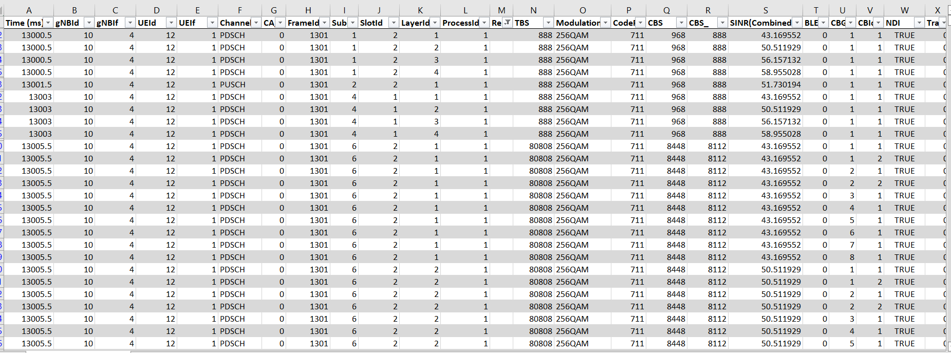
Figure 3‑11: HARQ log file showing code block transmission. Here CBS_ represents the information bits within a code block (CBS column).
-
Transmission attempts 1, 2, 3 and 4 are indexed as 0, 1, 2, 3. If the 4th attempt is errored, the CBG is dropped.
-
Packet trace only logs “packet” flow, and does not log flow of TBs, CBGs etc. Therefore, the packet trace logs a packet in the MAC OUT of the transmitter and subsequently if received successfully at the MAC IN of the receiver. If the packet errored, it is also marked in the packet trace.
-
Note that if a TB is in error than all the packets that were part of the TB will be marked as error.
-
The transmission/re-transmission of CBs is logged in the Code Block logfile.
-
The remarks column would have messages for HARQ preparation and would be blank for actual transmissions.
-
TBS is always logged on a per layer basis.
-
CBGID is also on a per layer basis
-
SINR reported in the CBG log is the post-soft combining SINR.

Figure 3‑12: HARQ log showing HARQ working via information provided in the Remarks columns
HARQ turn off#
There are ongoing discussions of abandoning of HARQ for the 1 ms end-to-end latency use case of URLLC. This decision implies that the code rate had to be lowered such that a single shot transmission, i.e., no retransmissions and no feedback, achieves the required BLER.
NetSim allows users to turn HARQ OFF via the GUI. Note that the code block log will continue to be written. Users will notice that errored CBGs are not retransmitted if HARQ is turned OFF. Since the CB/CBG is in error, that entire TB to which it belongs will be in error.
Users can inspect the packet trace and will see large numbers of packets errors if HARQ is turned OFF and if the UE is seeing a high BLER.
Segmentation of transport block into code blocks#
-
If the transport block size is larger than 3824, a 16-bit CRC is > added at the end of the transport block or 24-bit CRC is added.
-
The transport block is divided into multiple equal size code blocks > when the transport block size exceeds a threshold.
-
For quasi-cyclic low-density parity-check code (QC-LDPC) base graph > 1, the threshold is equal to 8448.
-
For QC-LDPC base graph 2, the threshold is equal to 3840. In 5G NR, > the maximum code block size number is 8448.
-
An additional 24-bit CRC is added at the end of each code block when > there is a segmentation.
-
A CBG can have up to 2/4/6/8 CBs.
-
Maximum transport block size - 1,277,992.
LDPC BG 1, CBS Max, (Kcb) = 8448, LDPC BG 2, CBS Max, (Kcb) = 3840

L = Extra CRC bits, C = Number of Code blocks, TBS = Size of Transport block, K′ = Information bits in code block. The base matrix expansion factor Zc is calculated by selecting minimum Zc in all sets of lifting size tables, such that: Kb × Zc ≥ K. Kb denotes the number of information bit columns for the lifting size Zc.
BLER and MCS selection#
NetSim GUI allows users set the BLER, via the BLER drop down option. This option has two settings, and each setting in-turn has different options for MCS selection. Both BLER and MCS selection are global options and will apply to all eNBs and UEs in both DL and UL in the network scenario.
-
Zero BLER
-
MCS Selection: Ideal Shannon theorem-based rate
-
Spectral efficiency is calculated assuming ideal Shannon rate > whereby
-
SpectralEfficiency = log2(1+SINR)
-
Spectral Efficiency - MCS Table 7.2.3-1 (4-bit CQI Table) of > standard 36.213 is looked up to select the MCS.
-
Data is transmitted at this MCS with zero BLER
-
MCS Selection: Shannon rate with attenuation factor
-
Spectral efficiency is calculated per the following expression > provided in TR 36.942:
SpectralEfficiency = α × log2(1+SINR)
-
α is the attenuation factor and generally 0.5 ≤ α ≤ 1.00. > Default: 0.75Spectral Efficiency - MCS Table 7.2.3-1 (4-bit CQI > Table) of standard 36.213 is looked up to select the MCS.
-
Data is transmitted at this MCS with zero BLER
PHY measurements#
All PHY measurements, downlink and uplink, are done on the actual transmitted data on the data channel. The measurements are not done using control the control channels.
The measurements are wideband i.e., a single value of channel state that is deemed representative of all RBs in use. This assumes that the PHY layer that the channel is flat across all the RBs. Such an assumption ensures acceptable accuracy for a system level simulation while keeping the computational complexity manageable.
The SNR in downlink (received by a UE from a eNB/gNB) and in the uplink (received by an eNB/gNB from a UE). The SNR is calculated at every slot and thereafter the SNR gets averaged after every "Average_SNR_Window" time frame to go forward and compute the AMC (Modulation & coding) information, and for each carrier as:
-
SNR = Received power / Thermal Noise.
-
Interference from other UEs / eNBs are not considered.
-
The received power is transmit power less propagation loss.
-
The MCS values are chosen based on the received SNR.
Carrier Aggregation#
Carrier aggregation is a feature that LTE-A uses to increase the bandwidth, and the bitrate. An aggregated carrier is known as a component carrier (CC). The component carrier can have a bandwidth of 1.4, 3, 5, 10, 15 or 20 MHz and a maximum of five component carriers can be aggregated. So, the maximum aggregated bandwidth is 100 MHz.
Carrier aggregation can be used: Frequency Division Duplex (FDD) and Time Division Duplex (TDD). The following figure illustrates the use of FDD.

Figure 3‑13: Illustrates the Carrier aggregation
FDD can use different number of component carriers in the Downlink (DL) and Uplink (UL). But, the number of UL component carriers must always be equal to or lower than the number of DL component carriers. Also, the individual component carriers can use different bandwidths.
TDD uses the same number of component carriers with identical bandwidths for DL and UL.
CA Configurations#
CA can be configured as into intra-band (contiguous and non-contiguous) and inter-band non-contiguous. Intra-band contiguous and inter-band combinations, that aggregate two Component Carriers (CCs) in downlink, are specified from Release 10.
The Intra-band contiguous CA configuration refers to contiguous carriers aggregated in the same operating band.
The Intra-band non-contiguous CA configuration refers to non-contiguous carriers aggregated in the same operating band.
The Inter-band CA configuration refers to aggregation of component carriers in different operating bands, where the carriers aggregated in each band can be contiguous or non-contiguous.
The following figure illustrates the CA configurations.
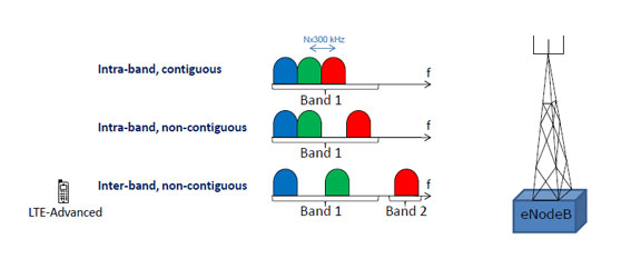
Figure 3‑14: Illustrates the CA configurations
CA Bandwidth Classes#
The following table lists the details of the Carrier Aggregation Bandwidth classes in terms of the total number of Resource blocks used by the CC.
For example, the Bandwidth class A specifies N_RB,agg \<= 100. This means that the Number of the aggregated RBs within the fully allocated Aggregated Channel bandwidth (NRB,agg) should be less than 100 and the aggregated Tx Bandwidth for class A cannot exceed 20 MHz, and limits to 1 CC in the band.
Note: NetSim currently supports CA Bandwidth classes A, B and C only.
| Class | Aggregated Transmission Bandwidth Configuration (ATBC) | Maximum # of CC | |
|---|---|---|---|
| NRB,agg | Maximum Tx bandwidth | ||
| A | N \<= 100 | 20 | 1 |
| B | 25 \< N \<= 100 | 20 | 2 |
| C | 100 \< N \<= 200 | 40 | 2 |
| D | 200 \< N \<= 300 | 60 | 3 |
| E | 300 \< N \<= 400 | 80 | 4 |
| F | 400 \< N \<= 500 | 100 | 5 |
| I | 700 \< N \<= 800 | 160 | 8 |
Figure 3‑15: CA Bandwidth classes
CA Configuration Naming Conventions#
To understand the naming conventions in a CA configuration and the bandwidth combination set usage, let us see the CA_1C configuration. This CA configuration states that the UE can operate on Band 1, with two continuous CCs and with a maximum of 200 RBs. The bandwidth combination set states that the allocation of those 200 RBs can be either 75 RBs on both CCs or 100RBs on both CCs.

Figure 3‑16: CA Configuration Naming Conventions
For more information about Carrier Aggregation, see
https://www.3gpp.org/technologies/keywords-acronyms/101-carrier-aggregation-explained.
CA Configuration Table (based on TR 36 716 01-01)#
Carrier aggregation can be configured in the eNB's Physical layer properties. Following are the various configuration options that are available as shown Table 3‑6 and Table 3‑7.
FDD Bands:
| CA Configuration Table | ||||||||
|---|---|---|---|---|---|---|---|---|
| CA Configuration | CA Count | CA Type | Frequency Range | Uplink Low (MHz) | Uplink High (MHz) | Downlink Low (MHz) | Downlink High (MHz) | |
| INTER_BAND_CA | ||||||||
| CA_1A_3A | 2 | CA1_UL, CA1_DL, CA2_UL, CA2_DL | FR1 | 1920, 1710 | 1980, 1785 | 2110, 1805 | 2170, 1880 | |
| CA_3A_7A | 2 | CA1_UL, CA1_DL, CA2_UL, CA2_DL | FR1 | 1710, 2500 | 1785, 2570 | 1805, 2620 | 1880, 2690 | |
| CA_3A_20A | 2 | CA1_UL, CA1_DL, CA2_UL, CA2_DL | FR1 | 1710, 832 | 1785, 862 | 1805, 791 | 1880, 821 | |
| CA_3A_28A | 2 | CA1_UL, CA1_DL, CA2_UL, CA2_DL | FR1 | 1710, 703 | 1785, 748 | 1805, 758 |
1880, 803 | |
| CA_3A_8A | 2 | CA1_UL, CA1_DL, CA2_UL, CA2_DL | FR1 | 1710, 880 |
1785, 915 | 1805, 925 | 1880, 960 | |
| CA_7A_20A | 2 | CA1_UL, CA1_DL, CA2_UL, CA2_DL | FR1 | 2500, 832 | 2570, 862 | 2620, 791 | 2690, 821 | |
| CA_7A_28A | 2 | CA1_UL, CA1_DL, CA2_UL, CA2_DL | FR1 | 2500, 703 |
2570, 748 | 2620, 758 | 2690, 803 | |
| CA_28A_32A | 2 | CA1_UL, CA1_DL, CA2_UL, CA2_DL | FR1 | 703, 1452 | 748, 1496 | 758, 1452 | 803, 1496 | |
| CA_1A_3A_7A | 3 | CA1_UL, CA1_DL, CA2_UL, CA2_DL, CA3_UL, CA3_DL | FR1 | 1920, 1710, 2500 | 1980, 1785, 2570 | 2110, 1805, 2620 | 2170, 1880, 2690 | |
| CA_3A_7A_20A | 3 | CA1_UL, CA1_DL, CA2_UL, CA2_DL, CA3_UL, CA3_DL | FR1 | 1710, 2500, 832 | 1785, 2570, 862 | 1805, 2620, 791 | 1880, 2690, 821 | |
| INTRA_BAND_CONTIGUOUS_CA | ||||||||
| CA_1C | 2 | CA1_UL, CA1_DL, CA2_UL, CA2_DL | FR1 | 1920, 1920 | 1980, 1980 | 2110, 2110 | 2170, 2170 | |
| CA_2C | 2 | CA1_UL, CA1_DL, CA2_UL, CA2_DL | FR1 | 1850, 1850 | 1910, 1910 | 1930, 1930 | 1990, 1990 | |
| CA_3B | 2 | CA1_UL, CA1_DL, CA2_UL, CA2_DL | FR1 | 1710, 1710 | 1785, 1785 | 1805, 1805 | 1880, 1880 | |
| CA_3C | 2 | CA1_UL, CA1_DL, CA2_UL, CA2_DL | FR1 | 1710, 1710 | 1785, 1785 | 1805, 1805 | 1880, 1880 | |
| CA_5B | 2 | CA1_UL, CA1_DL, CA2_UL, CA2_DL | FR1 | 824, 824 | 849, 849 | 869, 869 | 894, 894 | |
| CA_7B | 2 | CA1_UL, CA1_DL, CA2_UL, CA2_DL | FR1 | 2500, 2500 | 2570, 2570 | 2620, 2620 | 2690, 2690 | |
| CA_7C | 2 | CA1_UL, CA1_DL, CA2_UL, CA2_DL | FR1 | 2500, 2500 | 2570, 2570 | 2620, 2620 | 2690, 2690 | |
| CA_8B | 2 | CA1_UL, CA1_DL, CA2_UL, CA2_DL | FR1 | 880, 880 | 915, 915 | 925, 925 | 960, 960 | |
| CA_12B | 2 | CA1_UL, CA1_DL, CA2_UL, CA2_DL | FR1 | 699, 699 | 716, 716 | 729, 729 | 746, 746 | |
| CA_27B | 2 | CA1_UL, CA1_DL, CA2_UL, CA2_DL | FR1 | 807, 807 | 824, 824 | 852, 852 | 869, 869 | |
| CA_28C | 2 | CA1_UL, CA1_DL, CA2_UL, CA2_DL | FR1 | 703, 703 | 748, 748 | 758, 758 | 803, 803 | |
| CA_66B | 2 | CA1_UL, CA1_DL, CA2_UL, CA2_DL | FR1 | 1710, 1710 | 1780, 1780 | 2110, 2110 | 2200, 2200 | |
| CA_66C | 2 | CA1_UL, CA1_DL, CA2_UL, CA2_DL | FR1 | 1710, 1710 | 1780, 1780 | 2110, 2110 | 2200, 2200 | |
| CA_66D | 2 | CA1_UL, CA1_DL, CA2_UL, CA2_DL | FR1 | 1710, 1710 | 1780, 1780 | 2110, 2110 | 2200, 2200 | |
| CA_70C | 2 | CA1_UL, CA1_DL, CA2_UL, CA2_DL | FR1 | 1695, 1695 | 1710, 1710 | 1995, 1995 | 2020, 2020 | |
| INTRA_BAND_NONCONTIGUOUS_CA | ||||||||
| CA_1A_1A | 2 | CA1_UL, CA1_DL, CA2_UL, CA2_DL | FR1 | 1920, 1920 | 1980, 1980 | 2110, 2110 | 2170, 2170 | |
| CA_2A_2A | 2 | CA1_UL, CA1_DL, CA2_UL, CA2_DL | FR1 | 1850, 1850 | 1910, 1910 | 1930, 1930 | 1990, 1990 | |
| CA_3A_3A | 2 | CA1_UL, CA1_DL, CA2_UL, CA2_DL | FR1 | 1710, 1710 | 1785, 1785 | 1805, 1805 | 1880, 1880 | |
| CA_4A_4A | 2 | CA1_UL, CA1_DL, CA2_UL, CA2_DL | FR1 | 1710, 1710 | 1755, 1755 | 2110, 2110 | 2155, 2155 | |
| CA_5A_5A | 2 | CA1_UL, CA1_DL, CA2_UL, CA2_DL | FR1 | 824, 824 | 849, 849 | 869, 869 | 894, 894 | |
| CA_7A_7A | 2 | CA1_UL, CA1_DL, CA2_UL, CA2_DL | FR1 | 2500, 2500 | 2570, 2570 | 2620, 2620 | 2690, 2690 | |
| CA_12A_12A | 2 | CA1_UL, CA1_DL, CA2_UL, CA2_DL | FR1 | 699, 699 | 716, 716 | 729, 729 | 746, 746 | |
| CA_23A_23A | 2 | CA1_UL, CA1_DL, CA2_UL, CA2_DL | FR1 | 2000, 2000 | 2020, 2020 | 2180, 2180 | 2200, 2200 | |
| CA_25A_25A | 2 | CA1_UL, CA1_DL, CA2_UL, CA2_DL | FR1 | 1850, 1850 | 1915, 1915 | 1930, 1930 | 1995, 1995 | |
| CA_66A_66A | 2 | CA1_UL, CA1_DL, CA2_UL, CA2_DL | FR1 | 1710, 1710 | 1780, 1780 | 2110, 2110 | 2200, 2200 | |
| CA_66A_66B | 2 | CA1_UL, CA1_DL, CA2_UL, CA2_DL | FR1 | 1710, 1710 | 1780, 1780 | 2110, 2110 | 2200, 2200 | |
| CA_66A_66C | 2 | CA1_UL, CA1_DL, CA2_UL, CA2_DL | FR1 | 1710, 1710 | 1780, 1780 | 2110, 2110 | 2200, 2200 | |
| CA_25A_25A_25A | 3 | CA1_UL, CA1_DL, CA2_UL, CA2_DL, CA3_UL, CA3_DL | FR1 | 1850, 1850, 1850 | 1915, 1915, 1915 | 1930, 1930, 1930 | 1995, 1995, 1995 | |
| CA_66A_66A_66A | 3 | CA1_UL, CA1_DL, CA2_UL, CA2_DL, CA3_UL, CA3_DL | FR1 | 1710, 1710, 1710 | 1780, 1780, 1780 | 2110, 2110, 2110 | 2200, 2200, 2200 | |
| SINGLE_BAND | ||||||||
| BAND_1 | 1 | CA1 | FR1 | 1920 | 1980 | 2110 | 2170 | |
| BAND_2 | 1 | CA1 | FR1 | 1850 | 1910 | 1930 | 1990 | |
| BAND_3 | 1 | CA1 | FR1 | 1710 | 1785 | 1805 | 1880 | |
| BAND_4 | 1 | CA1 | FR1 | 1710 | 1755 | 2110 | 2155 | |
| BAND_5 | 1 | CA1 | FR1 | 824 | 849 | 869 | 894 | |
| BAND_6 | 1 | CA1 | FR1 | 830 | 840 | 875 | 885 | |
| BAND_7 | 1 | CA1 | FR1 | 2500 | 2570 | 2620 | 2690 | |
| BAND_8 | 1 | CA1 | FR1 | 880 | 915 | 925 | 960 | |
| BAND_9 | 1 | CA1 | FR1 | 1749.9 | 1784.9 | 1844.9 | 1879.9 | |
| BAND_10 | 1 | CA1 | FR1 | 1710 | 1770 | 2110 | 2170 | |
| BAND_11 | 1 | CA1 | FR1 | 1427.9 | 1447.9 | 1475.9 | 1495.9 | |
| BAND_12 | 1 | CA1 | FR1 | 699 | 716 | 729 | 746 | |
| BAND_13 | 1 | CA1 | FR1 | 777 | 787 | 746 | 756 | |
| BAND_14 | 1 | CA1 | FR1 | 788 | 798 | 758 | 768 | |
| BAND_17 | 1 | CA1 | FR1 | 704 | 716 | 734 | 746 | |
| BAND_18 | 1 | CA1 | FR1 | 815 | 830 | 860 | 875 | |
| BAND_19 | 1 | CA1 | FR1 | 830 | 845 | 875 | 890 | |
| BAND_20 | 1 | CA1 | FR1 | 832 | 862 | 791 | 821 | |
| BAND_21 | 1 | CA1 | FR1 | 1447.9 | 1462.9 | 1495.9 | 1510.9 | |
| BAND_22 | 1 | CA1 | FR1 | 3410 | 3490 | 3510 | 3590 | |
| BAND_23 | 1 | CA1 | FR1 | 2000 | 2020 | 2180 | 2200 | |
| BAND_24 | 1 | CA1 | FR1 | 1626.5 | 1660.5 | 1525 | 1559 | |
| BAND_25 | 1 | CA1 | FR1 | 1850 | 1915 | 1930 | 1995 | |
| BAND_26 | 1 | CA1 | FR1 | 814 | 849 | 859 | 894 | |
| BAND_27 | 1 | CA1 | FR1 | 807 | 824 | 852 | 869 | |
| BAND_28 | 1 | CA1 | FR1 | 703 | 748 | 758 | 803 | |
| BAND_30 | 1 | CA1 | FR1 | 2305 | 2315 | 2350 | 2360 | |
| BAND_31 | 1 | CA1 | FR1 | 452.5 | 457.5 | 462.5 | 467.5 | |
| BAND_65 | 1 | CA1 | FR1 | 1920 | 2010 | 2110 | 2200 | |
| BAND_66 | 1 | CA1 | FR1 | 1710 | 1780 | 2110 | 2200 | |
| BAND_68 | 1 | CA1 | FR1 | 698 | 728 | 753 | 783 | |
| BAND_70 | 1 | CA1 | FR1 | 1695 | 1710 | 1995 | 2020 | |
| BAND_71 | 1 | CA1 | FR1 | 663 | 698 | 617 | 652 | |
| BAND_72 | 1 | CA1 | FR1 | 451 | 456 | 461 | 466 | |
| BAND_73 | 1 | CA1 | FR1 | 450 | 455 | 460 | 465 | |
| BAND_74 | 1 | CA1 | FR1 | 1427 | 1470 | 1475 | 1518 | |
| BAND_85 | 1 | CA1 | FR1 | 698 | 716 | 728 | 746 | |
| BAND_87 | 1 | CA1 | FR1 | 410 | 415 | 420 | 425 | |
| BAND_88 | 1 | CA1 | FR1 | 412 | 417 | 422 | 427 | |
Table 3‑6: CA Configuration Table for FDD bands
TDD Bands:
| CA Configuration | CA Count | CA Type | Frequency Range | Uplink Low (MHz) | Uplink High (MHz) |
|---|---|---|---|---|---|
| INTER_BAND_CA | |||||
| DL_2A-48A_UL_2A-48A_BCS0 | 2 | CA1, CA2 | FR1 | 3550, 3550 | 3700, 3700 |
| DL_2A-48A-48A_UL_2A-48A_BCS0 | 2 | CA1, CA2 | FR1 | 3550, 3550 | 3700, 3700 |
| DL_2A-48A-48C_UL_2A-48A_BCS0 | 2 | CA1, CA2 | FR1 | 3550, 3550 | 3700, 3700 |
| DL_2A-48C_UL_2A-48A_BCS0 | 2 | CA1, CA2 | FR1 | 3550, 3550 | 3700, 3700 |
| DL_2A-48D_UL_2A-48A_BCS0 | 2 | CA1, CA2 | FR1 | 3550, 3550 | 3700, 3700 |
| DL_2A-48A-48D_UL_2A-48A_BCS0 | 2 | CA1, CA2 | FR1 | 3550, 3550 | 3700, 3700 |
| DL_2A-48E_UL_2A-48A_BCS0 | 2 | CA1, CA2 | FR1 | 3550, 3550 | 3700, 3700 |
| DL_2A-48A-48E_UL_2A-48A_BCS0 | 2 | CA1, CA2 | FR1 | 3550, 3550 | 3700, 3700 |
| INTRA_BAND_CONTIGUOUS_CA | |||||
| CA_3DL_41D_3UL_41D_BCS0 | 3 | CA1, CA2, CA3 | FR1 | 2496, 2496, 2496 | 2690, 2690, 2690 |
| CA_4DL_41E_3UL_41D_BCS0 | 4 | CA1, CA2, CA3, CA4 | FR1 | 2496, 2496, 2496, 2496 | 2690, 2690, 2690, 2690 |
| CA_5DL_41F_3UL_41D_BCS0 | 5 | CA1, CA2, CA3, CA4, CA5 | FR1 | 2496, 2496, 2496, 2496, 2496 | 2690, 2690, 2690, 2690, 2690 |
| 2DL_48C_2UL_48C_BCS0 | 2 | CA1, CA2 | FR1 | 3550, 3550 | 3700, 3700 |
| 3DL_48D_2UL_48C_BCS0 | 3 | CA1, CA2, CA3 | FR1 | 3550, 3550, 3550 | 3700, 3700, 3700 |
| 4DL_48E_2UL_48C_BCS0 | 4 | CA1, CA2, CA3, CA4 | FR1 | 3550, 3550, 3550, 3550 | 3700, 3700, 3700, 3700 |
| CA_48A_48B | 2 | CA1, CA2 | FR1 | 3550, 3550 | 3700, 3700 |
| CA_48B_48B | 2 | CA1, CA2 | FR1 | 3550, 3550 | 3700, 3700 |
| CA_48B_48C | 2 | CA1, CA2 | FR1 | 3550, 3550 | 3700, 3700 |
| CA_48B_48D | 2 | CA1, CA2 | FR1 | 3550, 3550 | 3700, 3700 |
| CA_48B_48E | 2 | CA1, CA2 | FR1 | 3550, 3550 | 3700, 3700 |
| INTRA_BAND_NONCONTIGUOUS_CA | |||||
| CA_2DL_42A-42A_1UL_BCS1 | 2 | CA1, CA2 | FR1 | 3400, 3400 | 3600, 3600 |
| CA_3DL_42A-42C_2UL_42C_BCS1 | 3 | CA1, CA2, CA3 | FR1 | 3400, 3400, 3400 | 3600, 3600, 3600 |
| CA_4DL_42C-42C_2UL_42C_BCS1 | 4 | CA1, CA2, CA3, CA4 | FR1 | 3400, 3400, 3400, 3400 | 3600, 3600, 3600, 3600 |
| 3DL_48A-48C_2UL_48C_BCS0 | 3 | CA1, CA2, CA3 | FR1 | 3550, 3550, 3550 | 3700, 3700, 3700 |
| 4DL_48C-48C_2UL_48C_BCS0 | 4 | CA1, CA2, CA3, CA4 | FR1 | 3550, 3550, 3550, 3550 | 3700, 3700, 3700, 3700 |
| SINGLE_BAND | |||||
| BAND_33 | 1 | CA1 | FR1 | 1900 | 1920 |
| BAND_34 | 1 | CA1 | FR1 | 2010 | 2025 |
| BAND_35 | 1 | CA1 | FR1 | 1850 | 1910 |
| BAND_36 | 1 | CA1 | FR1 | 1930 | 1990 |
| BAND_37 | 1 | CA1 | FR1 | 1910 | 1930 |
| BAND_38 | 1 | CA1 | FR1 | 2570 | 2620 |
| BAND_39 | 1 | CA1 | FR1 | 1880 | 1920 |
| BAND_40 | 1 | CA1 | FR1 | 2300 | 2400 |
| BAND_41 | 1 | CA1 | FR1 | 2496 | 2690 |
| BAND_42 | 1 | CA1 | FR1 | 3400 | 3600 |
| BAND_43 | 1 | CA1 | FR1 | 3600 | 3800 |
| BAND_44 | 1 | CA1 | FR1 | 703 | 803 |
| BAND_45 | 1 | CA1 | FR1 | 1447 | 1467 |
| BAND_46 | 1 | CA1 | FR1 | 5150 | 5925 |
| BAND_47 | 1 | CA1 | FR1 | 5855 | 5925 |
| BAND_48 | 1 | CA1 | FR1 | 3550 | 3700 |
| BAND_49 | 1 | CA1 | FR1 | 3550 | 3700 |
| BAND_50 | 1 | CA1 | FR1 | 1432 | 1517 |
| BAND_51 | 1 | CA1 | FR1 | 1427 | 1432 |
| BAND_52 | 1 | CA1 | FR1 | 3300 | 3400 |
| BAND_53 | 1 | CA1 | FR1 | 2483.5 | 2495 |
Table 3‑7: CA Configuration Table for TDD bands
Downlink Interference Model#
Configuration#
Downlink Interference Model can be configured in the eNB’s LTE interface properties under channel models section of Physical Layer as shown below:

Figure 3‑17: eNB >Interface (LTE) >Physical layer properties
Downlink Interference Model is set to NO_INTERFERENCE by default.
Graded distance-based Wyner model#
The Wyner model is widely used to model and analyze cellular networks due to its simplicity and analytical tractability. In this model:
-
Only interference from (two) adjacent cells is considered
-
Random user locations and path loss variations are ignored, and
-
The interference intensity from each neighboring base station (BS) is characterized by a single fixed parameter 0 ≤ 𝛼 ≤ 1). The channel gain between BS and its home user is 1 and the intercell interference intensity is 𝛼. Thus, a user sees a constant interference irrespective of its location.
These three simplifications lose a lot of information. We alter the Wyner model to address these flaws by:
-
Considering interference from arbitrary number of BSs
-
Factoring in the user location. The UEs distance from the interfering BS is an obvious factor that determines the interference intensity since the amount of interference caused depends on the signal attenuation with distance, the path loss law. Since the Wyner model uses relative interference, the ratio of a UEs distance from serving and interfering BSs is used as one of the interference parameters.
-
Using a graded interference intensity model, whereby a UE will see a different value of 𝛼 at different locations, thereby modelling the effect of interference more accurately.
Technical description#
-
We model DL interference from any number of interfering BSs. Let BSi be the serving BS to UEk. Let BSj be any other BS (j ≠ i). Then the distance between UEk and BSi is denoted as DUEkBSi, while the distance between UE and BSj is denoted as DUEkBSj.
-
A UE sees interference if > $\frac{\left( D_{UE_{K}}^{BS_{j}} - D_{UE_{K}}^{BS_{i}} \right)}{D_{UE_{K}}^{BS_{j}}}\ $is > within a user defined threshold (for example, 20%). This ratio is > also equal to > $1 - \frac{D_{UE_{k}}^{BS_{i}}}{D_{UE_{K}}^{BS_{j}}}$. When > DUEKBSi ≤ DUEKBSj, > we see that > $0 \leq \ \frac{\left( D_{UE_{K}}^{BS_{j}} - D_{UE_{K}}^{BS_{i}} \right)}{D_{UE_{K}}^{BS_{j}}} \leq 1$. > The ratio is 0 when > DUEKBSi = DUEKBSj > and is 1 when > DUEKBSi = 0. > When > DUEKBSi = DUEKBSj > the UE is equidistant from both BS i.e., at the cell edge. When > DUEKBSi = 0, > the UE is at the centre of the serving BS, BSi.
-
Users at the cell-edge will see out of cell interference; as the > user moves closer to the cell centre, it sees lesser interference.
-
We call this user defined threshold as differential distance ratio > threshold and denote it by DDRth. The DDR > threshold is used to define K thresholds, which are in turn used > to determine the out of cell interference experienced by > UEk, as explained below. First, we bin the > DDRth, conditional on > DUEKBSi ≤ DUEKBSj, > into K steps, as follows:
$$0 \leq \frac{\left( D_{UE_{K}}^{BS_{j}} - D_{UE_{K}}^{BS_{i}} \right)}{D_{UE_{K}}^{BS_{j}}} \< \left( \frac{{DDR}_{th}}{K} \right) \times 1\ $$
$$\left( \frac{{DDR}_{th}}{K} \right) \times 1\ \leq \ \frac{\left( D_{UE_{K}}^{BS_{j}} - D_{UE_{K}}^{BS_{i}} \right)}{D_{UE_{K}}^{BS_{j}}} \< \left( \frac{{DDR}_{th}}{K} \right)\ \times 2$$
…
$${\ldots }{\left( \frac{{DDR}_{th}}{K} \right) \times (K - 1) \leq \ \frac{\left( D_{UE_{K}}^{BS_{j}} - D_{UE_{K}}^{BS_{i}} \right)}{D_{UE_{K}}^{BS_{j}}} \< \left( \frac{{DDR}_{th}}{K} \right) \times K}$$
$$\left( \frac{{DDR}_{th}}{K} \right) \times K \leq \ \frac{\left( D_{UE_{K}}^{BS_{j}} - D_{UE_{K}}^{BS_{i}} \right)}{D_{UE_{K}}^{BS_{j}}}$$
Where DDRth, is a user input varying from 0.00 to 1.00 (default is 0.1 or 10%), and K, the number of steps, is a user input varying from 1 to 4 (default is 1).
-
The relative interference for each of these steps would be > In (0≤n≤K) where K is the number of steps and > n represents each individual step (n = p if the > pth inequality in the above is satisfied, > counting the first inequality as the zeroth inequality).
-
We specify the interference power relative to the power received > from BSi. Therefore, given the value of > In, interference power is calculated as the > received power from BSi (excluding beamforming > gain) less In. Thus
InterferencePowerfromBSj (dB)= ReceivedPowerfromBSi(dBm) − Inj(dB)
Therefore, we have Ini(dB)= PservingBS(dBm)− PInterferingBS(dBm). This is equivalent to the Wyner model with $\alpha = \frac{P_{Interfering}^{BS}}{P_{serving}^{BS}}$ in the linear scale; however, note that in our interference model, α depends on the UE’s location, because In depends on the distance.
- This interference powers (linear) from all interfering BSs are added to the noise power (in linear scale) and then
$$SINR = \ \frac{Received\ power\ from\ BS_{i} + BeamFormingGain}{\ NoisePower + \ \sum\ InterferencePower\ }$$
-
Each In is a user input. It is subject to the limits 0 ≤ In ≤ 20 dB. NetSim will enforce the sanity check 20≥ IK≥ IK − 1≥ …≥ I0 ≥ 0. Here IK is the relative interference seen when the UE is near BSi and I0 is the relative interference seen when the UE is nearly equidistant from its two nearest BSs (and hence far from BSi).
-
In an ideal case, when the user is at the cell edge, the received power from BSi will be roughly equal to the received power from BSj (since it is equidistant from the two BSs), and so SINRCellEdge will necessarily be less than 0 dB.
- As the UE moves away from the cell edge and towards > BSi, the received power from > BSi increases and that from > BSj decreases, and so the SINR improves. For > this reason, we have the limits on In as > 0 dB≤ In ≤ 20 dB. If the user sets > In to a large value, it will be equivalent to > having no inter-cell interference.
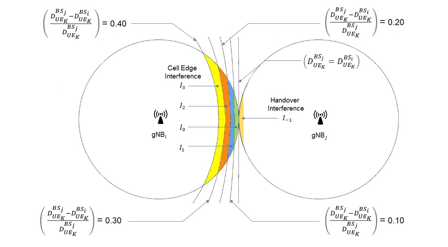
Figure 3‑18: Interference zones are the regions within the four curves and the cell boundary of gNBi. This example is for a case involving just 2 BSs with DDR = 0.4 and K = 4. The four curves are therefore the equations where $\frac{\left( \mathbf{D}_{\mathbf{U}\mathbf{E}_{\mathbf{K}}}^{\mathbf{B}\mathbf{S}_{\mathbf{j}}}\mathbf{-}\mathbf{D}_{\mathbf{U}\mathbf{E}_{\mathbf{K}}}^{\mathbf{B}\mathbf{S}_{\mathbf{i}}} \right)}{\mathbf{D}_{\mathbf{U}\mathbf{E}_{\mathbf{K}}}^{\mathbf{B}\mathbf{S}_{\mathbf{j}}}}$ is equal to $\frac{\mathbf{k}}{\mathbf{4}}\mathbf{= 0}\mathbf{.1,\ \ }\frac{\mathbf{2}\mathbf{k}}{\mathbf{4}}\mathbf{= \ 0.2,\ \ }\frac{\mathbf{3}\mathbf{k}}{\mathbf{4}}\mathbf{= \ 0.3}$, and $\frac{\mathbf{4}\mathbf{k}}{\mathbf{4}}\mathbf{= 0.4}$. The handover interference region is also shown.
-
In case $\frac{\left( D_{UE_{K}}^{BS_{j}} - D_{UE_{K}}^{BS_{i}} \right)}{D_{UE_{K}}^{BS_{j}}} > DDR_{th}$, the out of cell interference seen at the UE is set to IK. The default value of IK is 0, i.e., cell centre users do not see any out of cell interference. The default values of Ik for k = 1, 2, …, K − 1 is 10 dB.
-
In NetSim, handover is triggered when the signal strength from BSj is offset (3dB by default) higher than signal strength from BSi. A handover is not triggered when UEk is equidistant from both BSs but only when it is slightly nearer to BSj. Therefore, the short time when DUEKBSi ≥ DUEKBSj is a special case requiring a different interference power. We term this interference as “Handover interference” and is a separate user input. Handover interference is denoted as I−1 and − 3dB ≤ I−1 ≤ 0 dB.
Exact Geometric Model#
NetSim supports various 3GPP propagation models. These models are used to calculate the pathloss between every BS (eNB) and UE. One the parameters in the pathloss equations is the distance between the BS and the UE. Some of the other user settable parameters used in the 3GPP models are (i) Centre frequency (chosen from the band selected) (ii) Rural or Urban environments (iii) UE-BS channel is in LOS or NLOS (iv) Shadow-fading in the UE-BS channel (v) Indoor or outdoor UE location, etc., are also supported in NetSim.
Let BSi be the serving BS to UEk. Let BSj be any other BS (j ≠ i). UEk communicates with BSi while all other BSs (j ≠ i) act as interferers.
The distance between UEk and BSi is denoted as DUEkBSi, while the distance between UE and BSj is denoted as DUEkBSj. The power of the interfering signal from any BSj at any UEk depends on (i) the transmit power of the interfering BS and (ii) pathloss between the interfering BS and the UE. It can therefore be expressed as
IUEkBSj = PBSj − PLUEkBSj
where PBSj is the transmit power of BSj, PLUEkBSj represents the 3GPP model based pathloss between BSj and UEk. This pathloss is dependent on DUEkBSj and the channel between BSj and UEk. The interference powers (linear) from all interfering BSs (i.e., apart from the serving BS) are added to the noise power (in linear scale) and we get the expression
$$SINR_{UE_{k}} = \ \frac{Received\ power\ from\ BS_{i} + BeamFormingGain}{\ NoisePower + \ \sum_{j}^{}I_{UE_{k}}^{BS_{j}}\ \ }$$
The Wyner model is approximate but is computationally faster; the geometric model is precise but computationally slower due to the calculations involved.
Interference modeling in OFDM in NetSim#
NetSim doesn’t model the allocation of specific subcarriers to individual users. The aggregate resources are divided amongst the UEs per UEs’ requirements and the scheduling algorithm.
- The received power at UEk from BSi, with transmit power Pi is given (in the linear scale) as
$$P_{UE_{k}}^{BS_{i}} = \left( \frac{P_{i}}{PL_{UE_{k}}^{BS_{i}}} \right)$$
-
Iikj or the interference in linear scale at a UEk (associated with BSi) from BSj
-
To normalize the power should we further multiply by the ratio given below
$$I_{ik} = \Sigma_{j}\ I_{ik}^{j} \times \left( \frac{RB_{UE_{k}}^{slot}}{RB_{total}^{slot}} \right)$$
-
Assumptions:
-
The above formula assumes the interference seen by UEk is proportional to the number of RBs allotted to UEk
-
Fast fading is not accounted for in the interference calculations since it would require too much computational time, given that it needs to be re-calculated every coherence time.
-
- The total noise seen will be
k × T× RBUEkslot
- The signal power $P_{UE_{k}}^{BS_{i}} \times \left( \frac{RB_{UE_{k}}^{slot}}{RB_{total}^{slot}} \right)$
Therefore,
$$SINR = \frac{P_{UE_{k}}^{BS_{i}} \times \left( \frac{RB_{UE_{k}}^{slot}}{RB_{total}^{slot}} \right)}{k \times T \times \ RB_{UE_{k}}^{slot} + \ \Sigma_{j}\ I_{ik}^{j} \times \left( \frac{RB_{UE_{k}}^{slot}}{RB_{total}^{slot}} \right)\ }\ = \ \frac{P_{UE_{k}}^{BS_{i}}}{k \times T \times \ RB_{total}^{slot} + \ \Sigma_{j}\ I_{ik}^{j}\ }\ \ $$
Interference in MIMO#
- If UEk is receiving from BSi in multiple layers, the interference power Iikj is the same for all layers.
$$SINR_{L} = \ \frac{P_{UE_{k}}^{BS_{i}} \times \lambda_{L}}{k \times T \times \ RB_{total}^{slot} + \ \Sigma_{j}\ I_{ik}^{j}\ }$$
Where L represents a MIMO layer.
- Note that neither the noise nor the interference is divided by the layer count, because the combining vector has unit norm.
Limitations#
-
In the above interference formula NetSim assumes that all > interfering BSs transmit data in that slot.
-
The calculations need to be done for each slot. Enabling > interference in the UI will slow down the simulation.
Data rate calculation#
For NR, the approximate data rate for a given number of aggregated carriers in a band or band combination is computed as follows.
$$\text{Data\ rate\ }(\text{in\ Mbps}) = 10^{- 6} \cdot \sum_{j = 1}^{J}\left( v_{Layers}^{(j)} \cdot Q_{m}^{(j)} \cdot \ f^{(j)} \cdot R_{\max}\ .\frac{N_{PRB}^{BW(j),\mu} \cdot 12}{T_{s}^{\mu}}.\left( 1 - OH^{(j)} \right) \right)$$
wherein
J is the number of aggregated component carriers in a band or band combination.
Rmax = 948/1024
For the j-th CC,

Qm(j) is the maximum supported modulation order given by higher layer parameter supportedModulationOrderDL for downlink and higher layer parameter supportedModulationOrderUL for uplink.
f(j)is the scaling factor given by higher layer parameter scalingFactor and can take the values 1.
μ is the numerology (value is always 0)
Tsμ is the average OFDM symbol duration in a subframe for numerology μ, i.e. $T_{s}^{\mu} = \frac{10^{- 3}}{14 \times 2^{\mu}}$. Note that normal cyclic prefix is assumed.
NPRBBW(j), μ is the maximum RB allocation in bandwidth BW(j) with numerology μ
OH(j)is the overhead and takes the following values.
0.14, for frequency range for DL
0.08, for frequency range for UL
NOTE: Only one of the UL or SUL carriers (the one with the higher data rate) is counted for a cell operating SUL.
LTE Metrics#
LTE Packet trace#
The LTE packet trace file has in its column the field CNTROL_PACKET_TYPE. This field has control and data packets information, this field contains control packets related RRC connection (RRC_MIB, RRC_SIB1, RRC_SETUP_REQUEST, RRC_SETUP_COMPLETE, RRC_SETUP), UE_MEASUREMENT_REPORT, and STATUSPDU.

Figure 3‑19: Packet trace
Limitations#
NetSim’s LTE module has been developed a special case of the 5G NR library operating in the FR1 band with μ = 0. Hence some output metrics of 5G NR such as the SDAP metrics would appear in the LTE results. These can be ignored.
Reference Documents#
3GPP 36 series specifications for Long Term Evolution Networks.
3GPP TS 36.300 (Rel 10) Section 19.2.2.5
Latest FAQs#
You can refer to the up-to-date FAQs about NetSim’s LTE library at
https://tetcos.freshdesk.com/support/solutions/folders/14000107855