Introduction to modeling and simulation of networks#
A network simulator1 enables users to virtually create a network
comprising of devices, links, applications etc., and study the behavior
and performance of the Network.
Some example applications of network simulators are:
Protocol performance analysis
Application modeling and analysis
Network design and planning
Research and development of new networking technologies
Test and Verification
The typical steps followed when simulating any network are:
Building the model: Create a network with devices, links,
applications etc.
Running the simulation: Run the discrete event simulation (DES)
and log different performance metrics.
Visualizing the simulation: Use the packet animator to view the
flow of packets.
Analyzing the results: Examine output performance metrics such
as throughput, delay, loss etc. at multiple levels - network, link,
queue, application etc.
Developing your own protocol / algorithm: Extend existing
algorithms by modifying the simulator’s source C code.
NetSim is used by people from different areas such as industry, defense,
and academics to design, simulate, analyze and verify the performance of
different networks.
NetSim comes in three versions: Academic, Standard and Pro. The
academic version is used for lab experimentation and teaching. The
standard version is used for R&D at educational institutions while,
NetSim Pro version addresses the needs of defense and industry. The
standard and pro versions are available as
components in NetSim v13.2
from which users can choose and assemble. A comparison of the features
in the three versions are tabulated below Table 1‑1.
Features
Academic
Standard
Pro
Technology Coverage
Internetworks
Y
Y
Y
Legacy & Cellular Networks
Y
Y
Y
Advanced Routing
Y
Y
Y
Mobile Adhoc networks
Y
Y
Y
Software Defined Networks
Y
Y
Y
Wireless Sensor Networks
Y
Y
Y
Internet of Things
Y
Y
Y
Cognitive Radio Networks
Y
Y
Y
LTE Networks
Y
Y
Y
5G NR
N
Y
Y
VANET
N
Y
Y
Satellite Communication Networks
N
Y
Y
Underwater Acoustic Networks
N
Y
Y
TDMA
N
N
Y
Performance Reporting
Performance metrics available for Network and Sub-networks
Y
Y
Y
Packet Animator
Used to animate the packet flow in network
Y
Y
Y
Packet Trace
Available in tab ordered .csv format for easy post
processing
Y
Y
Y
Event Trace
Available in tab ordered .csv format for easy post
processing
N
Y
Y
Protocol Library Source Codes with Documentation
Protocol C source codes and appropriate header files with extensive
documentation
N
Y
Y
External Interfacing
Interfacing with SUMO
N
Y
Y
MATLAB
N
Wireshark
Y
Integrated debugging
Users can write their own code, link their code to NetSim and debug
using Visual Studio
N
Y
Y
Plots
Allows users to plot the value of a parameter over simulation
time
Y
Y
Y
Simulation Scale
100 Nodes
500 Nodes
~ 10,0000 Nodes
Custom Coding and Modeling Support
N
Y
Y
Emulator (Add on)
Connect to real hardware running live application
N
Y
Y
TDMA Radio Networks (Add On)
TDMA and DTDMA
N
N
Y
Target Users and Segment
Educational
(Lab Experimentation)
Educational
(Research)
Commercial
(Industrial and Defense)
Table ‑: A comparison of the features of NetSim Academic, Standard and
Pro versions
Components (Technology Libraries) in Pro and Standard versions#
Users can choose and assemble components (technology libraries) in
NetSim Standard and Pro versions as shown Table 1‑2.
Advanced Routing
Multicast Routing - IGMP, PIM, Access Control Lists, Detailed Layer 3
switch mode, Virtual LAN (VLAN), Public IP, Network Address Translation
(NAT)
IETF RFC’s 1771 & 3121
Component 4
Mobile Adhoc Networks
MANET - DSR, AODV, OLSR, ZRP
IETF RFC 4728, 3561, 3626
Component 5
Software Defined Network (SDN)
Based on Open Flow v1.3
Component 6
(Component 4 required)
Internet of things (IOT) with RPL protocol
Wireless Sensor Networks (WSN)
IEEE 802.15.4 MAC,
MANET in L3
RFC 6550
Component 7
Cognitive Radio Networks
WRAN
IEEE 802.22
Component 8
Long-Term Evolution Networks: LTE
3GPP
Component 9
(Component 4 required)
VANETs: IEEE 1609 WAVE, Basic Safety Message (BSM)
protocol per J2735 DSRC, Interface with SUMO for road traffic
simulation
IEEE 1609
Component 10
(Components 8 required)
5G NR :3GPP 38 Series. Full Stack covering SDAP,
PDCP, RLC – UM, TM, MAC, PHY – FR1 and FR2, mmWave propagation.
3GPP 38.xxx
Component 11
(Component 3 required)
Satellite Communication Networks: Geo Stationary
Satellite. Forward link TDMA in Ku Band and Return link MF-TDMA in Ka
band per DVB S2. Markov Loo Fading model. Device models for Satellite,
Satellite Gateway, and Satellite User Terminals
This is applicable when running Host-ID/ Dongle locked floating
licenses, and are not applicable for node locked licenses.
Any one system will have to be made as the license server, and it is to
this PC that the license is locked, either via its MAC ID or via a
dongle. The dongle is a USB device which controls the licensing. The
system(hardware/OS) requirements are same as that applicable for NetSim
clients. USB Port is required for connecting and running the
dongle. Client systems should be able to communicate with license server
through the network.
Install 64-bit build of NetSim. The start window will show (i) Version
type (Pro, Standard, Academic), (ii) Version Number and build number
(Eg: 13.3.11) followed by (iii) Currently supports 64bit in v13.3.
For example, you will see Network Simulator for a Standard version
to install. Double click on the setup file. Click on Yes button to
install the software.
Graphical user interface, application
Description automatically generated with medium confidence
Figure ‑: User Account Control message window appears and select Yes
button.
Setup prepares the installation wizard and software installation begins
with a Welcome Screen. Click on Next button to continue with the
installation.
Graphical user interface, application
Description automatically generated with medium confidence
Figure ‑: Select Next button to continue with the installation
License agreement will be displayed. Read the agreement carefully,
scroll down to read the complete license agreement. Click on I Agree
button else quit the setup by clicking Cancel button.
Graphical user interface, text,
application Description automatically generated
Figure ‑: Select I Agree button
If you agree with the license agreement, you will be prompted to select
either one of the installation options, Express (Single-click
installation) or Custom (Step-by-Step installation).
Express Installation will install the third-party tools silently along
with NetSim without displaying any prompts for the user.
Custom Installation is a step-by-step approach in which a user will be
prompted to carry out the installation process and the same applies to
the installation of the third-party tools which happens alongside
NetSim. Both the installation methods are explained below:
Graphical user interface, text,
application, email Description automatically generated
Figure ‑: Select Express (Single click) radio button and click on
install
NetSim installation starts, and users can see that the third-party tools
download information window click on OK to proceed with the
installation.
Figure ‑: Click on the OK button to proceed installation process of
NetSim
The third-party tools like Wireshark, SUMO, python, Winmerge, pywin, and
Microsoft.Net will begin to install. Before that, the installer will
look for the third-party tools at the same folder where NetSim.exe is
present if found, the next step of installation proceeds.
Else, the third-party tools will get downloaded from our NetSim servers
and installed if the PC/VM is connected to the Internet.
Graphical user interface, application
Description automatically generated
Figure ‑: Sumo is being downloaded
Graphical user interface, application,
table Description automatically generated
Figure ‑: python is being downloaded
Graphical user interface, application
Description automatically generated
Figure ‑: pywin is being downloaded
Graphical user interface, application
Description automatically generated
Figure ‑: Winmerge is being downloaded
Graphical user interface, application,
table Description automatically generated
Figure ‑: Wireshark is being downloaded
NetSim installation starts, and users can see that the third-party tools
get installed one by one.
Figure ‑: Wireshark gets installed silently
Figure ‑: Python gets installed silently
Figure ‑: Sumo gets installed silently
After the third-party installations, NetSim installation proceeds. Once
it is completed, NetSim-complete setup wizard appears as shown below.
Click on the Finish button to complete the installation process of
NetSim.
Figure ‑: Select Finish button to complete the installation process of
NetSim.
Graphical user interface, text,
application, email Description automatically generated
Figure ‑: Select Custom Radio button
Now the user will be prompted to select the components to be installed.
The list of components is available for selection and assembly only in
the Standard and Pro versions of NetSim. NetSim Academic version is
available as a single package.
Note: In Standard and Pro Versions of NetSim, the Choose Components
screen will display only those components for which the licenses are
obtained by the user. Also, Network Emulator and Real Time Protocol are
available as Add-On along with NetSim.
Graphical user interface, text
Description automatically generated
Figure ‑: list of components is available for selection and assembly
only in the Standard and Pro versions
Note: Select all the supporting applications for complete installation
of the software as shown below:
Click on the Next button.
Figure 2‑17: list of third-party tools
Note: Sumo, Python and Winmerge comes only as a part of Standard and Pro
Version Install.
In the next screen, you will be requested to enter the installation
path. Select the path in which the software needs to be installed and
click on Next button.
Figure ‑: NetSim installation directory path
In the next screen, you will be requested to enter the Start Menu folder
name. By default, it shows NetSim Standard for Standard version
install of NetSim. Click on the Install button to start the
installation.
Figure ‑: Start Menu folder name
The installation process begins.
Figure ‑: NetSim Standard v13.2 being installed.
After the installation of required NetSim files, the installation of
third-party tools begins.
For NetSim Academic Version, Npcap and Wireshark will be installed.
For NetSim Standard and Pro Versions, along with WinPcap and Wireshark
installation, Dot net, Sumo, Python installation will start
automatically. (If not deselected during 3rd party software selection)
If the PC/VM is connected to the Internet third party tools will get
downloaded from our NetSim servers (If the third-party tools are not
found in folder where NetSim.exe is present) and proceeds with
installation.
Click on Install button to start Dot NET (.NET) installation
Figure ‑: Select install button to install Dot NET (.NET)
Installation process begins.
Graphical user interface, application,
Teams Description automatically generated
Figure ‑: Dot NET (.NET) installation begins
Graphical user interface, application,
Teams Description automatically generated
Figure ‑: Dot NET (.NET) installation successfully completed
After the successful installation of Dot NET (.NET) and click on close
button then Wireshark installation window appears. Click on Next
button to begin
Figure ‑: Select Next button to start Wireshark installation
Wireshark License Agreement appears. Click on the I Agree
button.
Figure ‑: Wireshark License Agreement window
Make sure that all the components are selected and click on Next
button.
Figure ‑: Choose Wireshark features
Click on Next button.
Figure ‑: Select Next button
Select the path in which Wireshark needs to be installed and click on
Next button.
Figure ‑: Wireshark installation directory path
Select Install Npcap 0.995 and click on Next button.
Figure ‑: Select Install Npcap 1.55 in Wireshark window
Select Install USBPcap 1.3.0.0 and click on Install button.
Figure ‑: Select Install USBPcap 1.5.4.0 in Wireshark window
The installation process begins.
Figure ‑: Wireshark installation process begins
Npcap License Agreement window appears. Click on I Agree button and
proceed with the installation.
Graphical user interface, text,
application, email Description automatically generated
Figure ‑: Npcap License Agreement window
USBPcap Driver License Agreement window appears. Click on I accept the
terms of the License Agreement check box and click on Next button.
Figure ‑: USBPcap Driver License Agreement window
USBPcap CMD License Agreement window appears. Click on I accept the
terms of the License Agreement check box and click on Next button.
Graphical user interface, text,
application, email Description automatically generated
Figure ‑: USBPcap CMD License Agreement window
Figure ‑: USBPcap installation is completed
The Installation Complete dialog box appears once the installation
process is completed successfully. Click on the Next button
Graphical user interface, text
Description automatically generated
Figure ‑: Installation Complete dialog box and select next button
You will get the Wireshark Completing Setup window. Select the option
I want to manually reboot later.
Graphical user interface, application
Description automatically generated
Figure ‑: Select the option I want to manually reboot later and Click on
Finish button
This completes the Installation of Wireshark software. NetSim complete
Setup wizard appears as shown above. After click on Finish button to
begin with WinMerge installation.
Next the WinMerge License Agreement appears. Click on Next
button
Graphical user interface, text,
application, email Description automatically generated
Figure ‑: WinMerge License agreement window
Select the path in which WinMerge needs to be installed and click on
Next button
Graphical user interface, text,
application, email Description automatically generated
Figure ‑: Select the location where should WinMerge be installed
Once WinMerge installation completes, click on Finish button
Graphical user interface, application
Description automatically generated
Figure ‑: Click on Finish button to completes WinMerge installation
Click on Next button to start SUMO installation.
Graphical user interface, text,
application Description automatically generated
Figure ‑: Sumo Installation starts
SUMO License Agreement appears. Accept the terms in license
agreement and click on Next to proceed installation
Graphical user interface, text,
application, email Description automatically generated
Figure ‑: SUMO License Agreement window
Once SUMO installation completes, click on Finish button
Graphical user interface, application
Description automatically generated
Figure ‑: Complete SUMO Installation
Click on Next button to start with Python 3.7.4 installation.
Graphical user interface, text,
application Description automatically generated
Figure ‑: Select “install Now” option to install Python
The installation begins once you click on Install option.
Graphical user interface, text,
application Description automatically generated
Figure 2‑45: Python installation begins.
Graphical user interface, text,
application Description automatically generated
Once the installation is finished, click on Close button to start
the installation pywin 32
Graphical user interface, application
Description automatically generated
Figure ‑: pywin 32-224 installation wizard window
Click on Next button to select the directory to be used.
Graphical user interface, application
Description automatically generated
Figure ‑: Python directory path
Click on Next button to start the installation.
Graphical user interface, application
Description automatically generated
Figure ‑: Select Next button to install of pywin32
Once the installation is finished, click on Finish button.
Graphical user interface, application
Description automatically generated
Figure ‑: Select Finish button to complete pywin installation
This completes the Installation of pywin software. NetSim complete Setup
wizard appears as shown below. Click on Finish button to complete
the installation process of NetSim.
Graphical user interface, application
Description automatically generated
Figure ‑: NetSim complete Setup wizard
After this, to run NetSim, double click on the NetSim icon present in
the desktop or right click and choose Run as administrator option. A
NetSim License Server Information screen appears to start with NetSim.
Graphical user interface, application
Description automatically generated
Figure ‑: Enter NetSim License Server IP Address/Host name/Select NetSim
License file
Enter the NetSim License Server IP Address, i.e. the system in which
the License files are present and the rlm.exe file is running (Refer
Section 2.3.1 to set up NetSim License Server). In case of
Cloud/Node-locked/Evaluation license browse the provided LIC file and
click on OK button. Once this is done, NetSim Home screen will appear.
Steps for silent installation in NetSim are as follows.
For example, let us take the
NetSim_Standard_13_2_34_HW_64bit.exe setup. Right click on
NetSim Standard 64-bit setup à Go to properties and copy the
Location as shown below.
Figure 2‑53: NetSim Standard 64-bit setup location
Open command prompt and paste the copied location as shown below.
Figure 2‑54: Enter setup location in command prompt
Run/Execute Command with the following parameters:
NetSim_Standard_13_3_11_HW_64bit.exe/S /silent=1
>\<setup location/S\<space>/silent=1
silent=1: It will install NetSim and third-party tools silently.
/S: It will Install NetSim itself silently.
Figure ‑: Silent installation command in command prompt
Press the Enter key. The following User Account Control message
window appears. Click on Yes button to begin silent installation
of NetSim.
Graphical user interface, application
Description automatically generated with medium confidence
Figure 2‑56: User Account Control message window appears and select Yes
Note: Complete installation of NetSim may take up to 2 or 3 minutes.
Installing NetSim RLM Dongle Driver Software (Dongle Based Licenses)#
This section guides you to install the RLMDongle Driver software
from the CD-ROM.
Insert the CD-ROM disc in the CD drive.
Double click on My Computer and access the CD Drive.
Double click on Driver_Software folder.
Double click on HASPUserSetup.exe
Each prompt displayed during the process tells you what it is about to
do and prompts to either continue or exit.
Setup prepares the installation wizard and the driver software
installation begins with a Welcome Screen. Click on Next button.
Figure ‑: Sentinel Runtime Setup window and select Next button
Note: Any other program running during the installation of the Dongle
will affect the proper installation of the software.
Sentinel Runtime Setup License Agreement appears. Read the license
agreement carefully, scroll down to read the complete license agreement.
If the requirement of the license agreement is accepted, Click on I
accept the license agreement and click on Next button else quit the
setup by clicking Cancel button.
Figure 2‑58: Sentinel Runtime Setup License Agreement window appears and
select Next button
The installation process begins.
Figure 2‑59: Installation process begins
Once the Sentinel Runtime is installed successfully, click on Finish
button.
Figure 2‑60: Sentinel Runtime is installed successfully and select
Finish button
Now the RLM driver software is installed successfully. If the driver has
been successfully installed, then upon connecting the Dongle in the USB
port, a red light will glow (Refer picture below Figure 2‑61). If the
driver is not properly installed, this light will not glow when the
dongle is connected to the USB Port.
Figure 2‑61: Connecting the Dongle in the USB Port
Copy the NetSim License Server folder and paste it on
Desktop. Check that it has the license file. If not copy the
paste the license file into the License server folder
Double click on NetSim License Server folder from Desktop.
Double click on rlm.exe
For hardware dongle-based users: After the Driver Software
installation, connect the RLM dongle to the system USB port.
Double click on My Computer and access the CD Drive. This CD
contents will have the NetSim License server folder.
Note: For running NetSim, rlm.exe must be running in the server (license
server) system and the server system IP address must be entered
correctly. Without running rlm.exe, NetSim won’t run.
While running rlm.exe, the screen will appear as shown below Figure
2‑62.
Figure ‑: When NetSim license server system running, window appears
After running rlm.exe, double click the NetSim icon in the Desktop. The
screen given below will be obtained. Enter the Server IP address where
the rlm.exe is running and click OK.
Graphical user interface, application
Description automatically generated
The graphical user interface (GUI) allows users to interact with the
simulator for creating, modifying and saving, simulation experiments and
workspaces. This is much easier to use when compared to command line or
text-based simulator interfaces. NetSim GUI comprises of the Home
Screen, Design Window, Results Window, Animation Window and Plots
Window.
You see the NetSim Home Screen when you run NetSim software for the
first time, after checking out a license from the NetSim License Server.
See the following image for an example of the NetSim Home screen as
shown below Figure 3‑1.
Figure 3‑1: NetSim Home screen
You see the following items on the NetSim Home screen:
New Simulation: Use this menu to simulate different types of
networks in NetSim. You can simulate the following the types of
networks: Internetworks, Legacy Networks, Mobile Adhoc networks,
Cellular Networks, Wireless Sensor Networks, Internet of Things,
Cognitive Radio Networks, LTE/LTE-A Networks, 5G NR, VANETs,
Satellite Communication and Underwater Network (newly added
component in v13). Only the networks (components) for which licenses
are available will be shown. The networks (components) shown at the
bottom with grey background cannot be directly clicked and entered.
These features can be accessed through other components given the
dependencies.
Your work: Use this menu to load saved configuration files from
the current workspace. You can view, modify or re-run existing
simulations. Along with this, users can also export the saved files
from the current workspace to their preferred location on their
PC’s.
Examples: Use this menu to perform simulations of different
kinds categorized technology-wise. Users can choose any network
which they want to work. Expand and click on file name to display
simulation examples. Then click on a tile in middle panel to load
simulation, users can run and analyze the results. Users can click
on the book icon present in the right-hand side of each network
which opens the corresponding pdf files. This helps the users with
all information about the current simulation as well as the entire
network technology.
Figure ‑: Featured Examples List Window
Experiment: Users can use this menu to find experiments section
which has various experiments covering all the technologies in
NetSim. Users can choose their experiment by Expand and click on
file name to display the experiment. Then click on a tile in middle
panel to load simulation. All the settings to carry out the
experiment are already done. Users can click on the book icon
present in the right-hand side of each experiment. This will open
the corresponding pdf file for the experiment which consists of
detailed description of that experiment.
Figure ‑: Experiments List Window
License Settings: Use this menu to perform the following. Click
on License Settings provides users with three sub-menus related to
License information.
License Server Information: Use this menu to view details about the
NetSim License Server from where the client is checking out licenses.
Graphical user interface, text,
application, email Description automatically generated
Figure ‑: NetSim License Server Information window
You will see the following details on the NetSim Home screen, if you
click the License Server Info menu item: the type of platform on which
NetSim is running, the version of RLM, the Dongle RLM ID, the IP address
of the NetSim License Server, and the path to the license files in the
server hosting NetSim License Server.
End User License Agreement: Use this menu to view the end user
license agreement. You will see the following details on NetSim Home
screen, if you click the End User License Agreement menu item: Grant of
License and Use of the Services, License Restrictions, License Duration,
Upgrade and Support Service etc.
Configure Installed Components/Libraries: Use this menu to allow
NetSim users to simulate only specific types of networks (by the
licenses and libraries associated with the types of networks). You
control access to types of networks by selecting libraries for specific
types of networks that NetSim License Server checks out when NetSim
users start NetSim.
NetSim Home screen displays libraries for components for which you have
purchased licenses.
Note: You can select or clear libraries and control access to NetSim
users, only if you are using floating licenses.
See the following image for an example of what the NetSim Home screen
displays, if you click the Configure Installed Components/Libraries menu
item.
Graphical user interface, application,
email Description automatically generated
Figure ‑: The Installed Component (Libraries) of NetSim
Use the License Settings menu as follows:
Select the checkboxes for the component libraries (types of
networks) that NetSim users must be allowed to simulate.
Clear the checkboxes for the component libraries (types of networks)
that NetSim users must not be allowed to simulate.
The Internetwork component is greyed out. You cannot clear the
Internetworks component because Internetworks is a base component that
is required for all the other components to work.
Exit: Use this option to close opened Netsim tabs.
Support: Use this section to reach TETCOS LLP helpdesk.
Contact Technical Support link can be used to raise a trouble
ticket, you can also write to us via Email to
support@tetcos.com, and
Answers/FAQ link grants you access to our Knowledge Base
which contains answers to all your questions most of the time. Users
can utilize the wealth of information present in it, which are
further classified into the following: FAQs, Technologies/Protocols,
Modelling/UI/Results, and Writing your own code in NetSim.
Learn: Use this section to learn more about the software which
includes the following: Videos section can be used to view
videos related to NetSim in TETCOSLLP YouTube channel. This
channel helps users by providing frequent updates on what’s new in
NetSim, topics related to various network technologies covering
different versions of NetSim, and monthly webinars. The
Experiments Manual section grants you access to a well-designed
experiments manual covering various networking concepts which helps
users to easily understand different networks and also gain ideas to
carry out their own experimentations in NetSim.
Documentation: Use this section to open the following NetSim
help documents: These include the User Manual which consists of
complete description about all the features in NetSim and how it can
be used by the end users, the Technology Libraries which
provides users with an access to a detailed description of various
Network Technologies present in NetSim through individual pdf files,
and Source code help which comes along with Standard and Pro
Versions of NetSim, allows users to gain a better understanding of
the underlying code structure for in-depth analysis.
Contact Us: Use this section to contact us and know more
information about our product. You can write to us via Email to
sales@tetcos.com or contact us via Phone to our official
number +91 76760 54321.
Website: Use this link www.tetcos.com
to visit our website which consists of vast information that will assist
you through all walks of NetSim.
The Simulation window loads up once user selects the desired network
technology from the New Menu. Click on New Simulation and select the
desired kind of network to simulate.
Application Description automatically
generated with low confidence
Figure ‑: NetSim Home Screen
Save
Figure ‑: To save experiment, Select File >Save. Save As etc
To save experiment, select File à Save, then specify the Experiment
Name, Description (Optional) and click Save. The short cut for the same
is Ctrl + S.
Save as
To save an already existing/saved experiment by a different name after
performing required modifications/changes to it (without overwriting the
existing copy), Save As option can be used. Select File à Save As, then
specify the Experiment Name, Description (Optional) and click Save. The
short cut for the same is Shift + Ctrl + S and F12.
The settings menu provides user’s access to the simulation environment
settings.
Graphical user interface, text
Description automatically generated
Figure ‑: Environment settings
The Environment Settings window is used to switch between Grid View and
Map View backgrounds in supported network technologies. For Grid view,
users can configure the Grid environment length in meters as shown
Figure 3‑9.
This section will demonstrate how to create a basic network scenario and
analyze the results. Let us consider Internetworks. To create a new
scenario, Go to New Simulation à Internetworks as shown below Figure
3‑13.
A screenshot of a computer Description
automatically generated
In this example, a network with two subnets is designed. Let us say the
subnet 1 consists of two wired nodes connected via a Switch and the
other subnet consists of one wired node. Both the subnets are connected
using a Router. Traffic in the Network flows from a wired node in subnet
1 to the wired node in subnet 2.
Figure ‑: Network Topology in this experiment
Perform the following steps to create this network design.
Step 1: Drop the devices. Click on Node icon and select à Wired
Node.
Figure ‑: Internetworks Device Palette in GUI
Click on the environment (the grid) where you want the Wired Node to be
placed. In this way, place two more wired nodes. Similarly, to place a
Switch and a Router, click on the respective device and click on the
environment at the desired location.
Figure ‑: Dropped Devices on GUI
Note that NetSim takes the (x, y) position of any device on the grid is
the position of top left corner of the icon and not the center of the
icon.
Step 2: Connecting devices: Select the link and then left click on
one device, free the mouse button, then click on the second device and
free the mouse button. The wired links may disappear if you right click
anywhere in the environment. Clicking and dragging without freeing the
mouse pointer would displace the device in the environment.
Figure ‑: To Connect devices select wired/wireless links
For example, select link and the click on Switch followed by router to
connect them. In this manner, continue to link all devices.
In NetSim, users can Turn-On or Turn-Off display information such as IP
Address of the devices, link speed etc. For doing this click on Display
settings as shown below Figure 3‑22.
Graphical user interface Description
automatically generated with medium confidence
Figure ‑: Turn-On or Turn-Off display information such as IP Address of
the devices, link speed etc
In NetSim the device ID serves as a “device identifier” while the IP
Address is an “Interface identifier”
In NetSim simple copy paste can be used. Using this feature users can
copy all the properties of a device and create a new device with similar
properties.
Right click on the device, click on copy and then right click and click
paste. The sequence is shown below Figure 3‑23/Figure 3‑24/Figure
3‑25/Figure 3‑26/Figure 3‑27.
Figure ‑: Devices present on GUI
Figure ‑: Right click on the user device and Select copy.
Figure ‑: Right click on the GUI and Select Paste
Figure ‑: Devices Pasted in GUI
Remove in the device options, is used to delete the device from the grid
environment. Given below is an example of removing the device
User_Device_4 which was previously pasted.
Figure ‑: Right click on User_Device_4 and Select Remove
After the network is configured, user needs to model traffic from Wired
Node 2 to Wired Node 3. This is done using the application icon. Click
on the Application icon present on the ribbon as shown below Figure
3‑28.
Figure ‑: Select Application icon present on ribbon
In screen shot shown below the Application type is set to CBR, Source_ID
is 2 and Destination_ID is 3. Click on OK.
Packet and Event Trace files are useful for detailed simulation
analysis. By default, these are not enabled since it slows down the
simulation. To enable logging of Packet Trace, click on the icon in the
tool bar and to enable Event trace, click on the options in the ribbon
as shown below. Set the file name and select the required attributes to
be logged. For more information, please refer sections 8.4 and
8.5 respectively.
During Simulation: Users can save by using the short cut CTRL + S.
After Simulation: From Network Window: Click on File > Save button
on the top left. Next, specify the Experiment Name, Description
(Optional) and click on Save.
Graphical user interface, text,
application Description automatically generated
Figure ‑: Save popup window
Upon saving several files would get saved inside the folder, including:
NetSim keyboard shortcuts can be used for frequently performed tasks.
The keyboard shortcuts that are currently supported are listed in the
table below Table 3‑1.
Keys
Function
Home Screen
Ctrl + N
Open a New Network
Ctrl + O
Open a Saved Network
Design Window (Any Network)
Ctrl + C
Copy
Ctrl + V
Paste
Ctrl + R
Open Run Simulation Window
Ctrl + S
Save the Experiment
Shift + Ctrl + S
Save As (To Save under different name)
Ctrl + P
Open Image/Screenshot of the network scenario that is designed in the GUI
Alt+ F4
Close Window
F1
User Manual Help
Ctrl + '+/-'
Zoom In/Zoom Out
Mouse Click (Left)
Select a device
Ctrl + A
Select All devices in the design environment
Ctrl + Mouse Click (Left) and Drag
Select devices within a selected area
Delete
Deletes the selected devices in the Environment along with any links it may have
Simulation Console
Ctrl + C
Terminates Simulation in Mid way. Results will be calculated till the time at which the simulation is terminated
NetSim allows users to interact with the simulation at runtime via a
socket or through a file. User Interactions make simulation more
realistic by allowing command execution to view/modify certain device
parameters during runtime.
This section will demonstrate how to perform Interactive simulation for
a simple network scenario. Let us consider Internetworks. To create a
new scenario, go to New à Internetworks. Click & drop Wired Nodes and
Router onto the Simulation Environment and link them as shown below
Figure 3‑35.
Figure ‑: Network Topology
Click on Application icon present in the top ribbon and set the
Application type as CBR. The Source_Id is 1 and Destination_Id is 2.
Set Start Time as 30 Sec
Enable Plots and Packet trace options
Click on run simulation option and In the Run time Interaction tab
set Interactive Simulation as True and click on Accept as shown
below Figure 3‑36.
Figure ‑: Run time Interaction tab set Interactive Simulation as True
Click on run simulation and set Simulation Time as 500 sec. (It is
recommended to specify a longer simulation time to ensure that there
is sufficient time for the user to execute the various commands and
see the effect of that before Simulation ends) and click OK.
Simulation (NetSimCore.exe) will start running and will display a
message “waiting for first client to connect” as shown below Figure
3‑37.
C:\Users\TETCOS_PC\Desktop\Capture.PNG
Figure ‑: Waiting for first client to connect
After Simulation window opens, goto Network scenario and right click
on Router_3 or any other node and select NetSim Console option as
shown Figure 3‑38.
Figure ‑: Select NetSim Console option
Now client (NetSimCLI.exe) will start running and it will try to
establish connection with NetSimCore.exe. After connection is
established, the window will look similar like this shown below
Figure 3‑39.
C:\Users\TETCOS_PC\Desktop\Capture.PNG
Figure ‑: Connection is established
After this the command line interface can be used to execute the
supported commands
Note: Commands are not case sensitive
Simulation specific (Not applicable for file based interactive simulation)#
Pause
Pause At
Continue
Stop
Exit
Reconnect
Pause: To pause the currently running simulation
PauseAt: To pause the currently running simulation with respect to
particular time (Ex: To Pause simulation at 70.2 sec use command as
PauseAt 70.2)
Continue: To start the currently paused simulation. When a user
pauses simulation and then continue using the pause/continue commands,
it may appear as if simulation was running in the background. This is
not true. When interactive simulation is run, the simulation clock in
NetSim is Min (Wall Clock, Simulation Clock). Thus, before pausing
simulation may have been running at Wall clock (real time) speed even
though the simulation could have run much faster. On typing the
continue command simulation will run at it usual (much faster) speed
till it equals Wall clock (Real time). This behaviour sometimes can be
confusing to users.
Stop: To stop the currently running simulation (NetSimCore.exe)
Exit: To exit from the client (NetSimCLI.exe)
Reconnect: To reconnect client (NetSimCLI.exe) to simulation
(NetSimCore.exe) when we rerun simulation again
In order to view the entire contents of the IP routing table, use
following commands route print.
route print
Figure ‑: Network Route Print
You will see the routing table entries with network destinations and
the gateways to which packets are forwarded when they are headed to
that destination. Unless you’ve already added static routes to the
table, everything you see here will be dynamically generated.
In order to delete route in the IP routing table you will type a
command using the following syntax
Route delete destination_network
So, to delete the route with destination network 11.5.1.2, all we’d
have to do is type this command.
route delete 11.5.1.2
To check whether route has been deleted or not check again using
route print command.
To add a static route to the table, you will type a command using
the following syntax.
route ADD destination_network MASK subnet_mask gateway_ip METRIC
metric_cost IF interface_id
So, for example, if you wanted to add a route specifying that all
traffic bound for the 11.5.1.2 subnet went to a gateway at 11.5.1.1
route ADD 11.5.1.2 MASK 255.255.0.0 11.5.1.1 METRIC 100 IF 2
If you were to use the route print command to look at the table
now, you would see your new static route.
Figure ‑: Route added into Network
Note: Entry added in IP table by routing protocol continuously gets
updated. If a user tries to remove a route via route delete command,
there is always a chance that routing protocol will re-enter this entry
again. Users can use ACL / Static route to override the routing protocol
entry if required.
Routers provide basic traffic filtering capabilities, such as blocking
Internet traffic, with access control lists (ACLs). An ACL is a
sequential list of permit or deny statements that apply to addresses or
upper-layer protocols. These lists tell the router what types of packets
to: permit or deny. When using an access-list to filter traffic, a
permit statement is used to “allow” traffic, while a deny statement is
used to “block” traffic.
ACL Commands
To view ACL syntax use: acl print.
Before using ACL’s, we must first verify that acl option enabled. A
common way to enable ACL use command: acl enable.
Enters configuration mode of ACL using: aclconfig
To view ACL Table: Print
To exit from ACL configuration use command: exit
To disable ACL use command: acl disable (use this command
after exit from acl configuration)
To view ACL usage syntax use: acl print
[PERMIT, DENY] [INBOUND, OUTBOUND, BOTH] PROTO SRC DEST SPORT
DPORT IFID
The impact of ACL rule applied over the simulation traffic can be
observed in the IP_Metrics_Table in the simulation results window, In
Router_3 number of packets blocked by firewall has been shown below.
Note: Results will vary based on time of ACL command are executed
Figure ‑: IP Metrics Table in result window
Check Packet animation window whether packets has been blocked in
Router_3 for period when the ACL rule is applied. In the Below figure
you can observe that packets are getting discarded at Router_3.
Figure ‑: NetSim Animation Window when ACL rules are applied
Then packet transmission is allowed through same Interface_3 once after
ACL is disabled.
Figure ‑: NetSim Animation Window After ACL Disabled
The impact of ACL rule applied over the simulation traffic can be
observed in the Application throughput plot. Throughput graph will show
a drop after ACL is set. If ACL is disabled after a while, application
packets will start flowing across the router. The Application throughput
plot will show a drop and increase(Moving througput graph) in throughput
after setting ACL and disabling ACL respectively.
Example: ACL rule applied at around 120sec user can see the drop in
throughput in the graph, since router blocks UDP packets in the plot.
Once ACL has been disabled at around 185sec router permits packets and
hence increase in throughput can be observed in the plot shown below
Figure 3‑51.
Interactive simulation using file allows users to pass commands as input
through a text file. In the text file users can provide the commands
along with the device in which it has to be executed by specifying the
time stamps. This provides the user to have control over the scenario to
execute commands at a specified time.
In the Interactive simulation text file, user should specify the exact
time in seconds, along with the name of the device.
Format of the input text file for one device.
TIME=\<SIMULATION TIME IN SECONDS>
DEVICE=\<DEVICE_NAME>
\<COMMAND TO BE EXECUTED>
The below Network scenario explains how to perform the Interactive
simulation using file as input.
Figure ‑: Network Topology
The scenario comprises of 4 Routers, 2 Wired Node
In the Router Application layer, the routing protocol is set as RIP,
since it is global property, routing protocol will be set as RIP in
all Routers.
Right click on the Application Flow App1 CBR and select Properties
or click on the Application icon present in the top ribbon/toolbar.
A CBR Application is generated from Wired Node 1 i.e., Source to
Wired Node 2 i.e., Destination with Packet Size remaining 1460Bytes
and Inter Arrival Time remaining 20000µs. Transport Protocol is set
to UDP.
Additionally, Set start time as 1 sec.
To set static routes to forward packets from Router 3 to the
destination Wired Node via Router 5 instead of Router_4, such that
the packets flow from Router 3=> Router 5=>Router 6=>Router4
=>Wired node 2 from a specified time say 25 seconds, the following
input can be provided:
TIME= 25
DEVICE=Router_3
route ADD 11.5.1.2 MASK 255.255.255.0 11.2.1.2 metric 1 if 2
Create a text file with the above input and save it as input.txt
file.
Enable packet trace and Open the Run tab and switch to run time
simulation tab select the Interactive simulation using file.
Figure ‑: Run time Interaction tab with Interactive Simulation option
set as True (Using File)
Browse the Saved input.txt file in file path and select Accept
> button.
Figure ‑: Run time Interaction tab with Interactive Simulation File Path
set
Open the packet trace, you can observe that till 25 seconds the data
packets are transmitted from Wired Node 1=>Router 3=> Router 4=>
Wired Node 2.
Figure ‑: Data packets are transmitting from Wired Node 1=>Router 3=>
Router 4=> Wired Node 2 in packet trace before 25th seconds
After 25th second you can observe that, the routing
happens according to the command specified in the input file.
The data (APP 1 CBR) packets are transmitted from Wired Node
1=>Router 3=>Router 5=>Router 6=>Router 4=>Wired Node 2
Figure ‑: After 25th sec routing is initiating according to the command
mentioned in input file
The same can be observed in Animation window.
Figure ‑: NetSim Animation window
From the above example we can see that until the specified time
mentioned in the input text file, the network considers the path
formed by the routing protocol i.e RIP. From 25th Second onwards
packets are routed according to the modified path specified in
interactive simulation input text file.
NetSim provides run-time interfacing with Python so that users who are
familiar with python can implement some parts of their algorithm in
Python without having to modify the C source codes of NetSim. A lot of
work related to machine learning, artificial intelligence, and
specialized mathematical algorithms which can be used for networking
research, can be carried out using Python code.
NetSim offers Socket interfacing to interact with Python during runtime.
Connections are made using the port and IP address/Loopback address of
the system running NetSim.
NetSim provides a TCP socket with which a socket program/application
written in any programming language can establish a connection. The
conversation can remain until the connection is terminated by either
side.
By default, NetSim uses the port 8999 in which it listens for any
incoming connections. Client programs can connect to the NetSim socket
using the loopback/IP address of the system running NetSim along with
the port number 8999.
A client socket program written in Python can connect to the NetSim
Server process in a similar way as depicted here using the loopback
address 127.0.0.1 and port 8999.
After users design and simulate a network in NetSim it can be saved as
an experiment. This experiment is saved in a Workspace. A workspace
also contains the source codes, executable files, icons, data files,
etc. A workspace can contain one or more experiments. While NetSim
supports multiple workspaces, users generally work in the default
workspace. The default workspace of NetSim will have the master source
code and the master binaries (compiled library, executable and DLL
files).
New workspaces need to be created when:
The user wants to modify the underlying source code of NetSim.
A user chooses to organize a large number of saved experiments. The
experiments can be saved in a different workspace.
NetSim running on one PC/VM is time-shared between multiple users.
Each user has his/her own workspace.
As mentioned earlier, NetSim stores your experiments (projects) in a
folder termed as a Workspace. Default workspace is created in a user
selected directory when NetSim is run for the first time after
installation. Choose the path and enter the workspace name where you
want the default workspace to be created.
Graphical user interface, text,
application, email Description automatically generated
Figure ‑: Default workspace created in Documents folder
This default workspace contains the following folders:
\src - contains protocol source codes.
\bin_x64 contains NetSim binaries for 64-bit.
Graphical user interface, text,
application Description automatically generated
Figure ‑: Default workspace containing the different folders
Note: In NetSim, the default workspace cannot be renamed.
How does a user create and save an experiment in a workspace?#
To create an experiment, select New Simulation - \<Any Network> in the
NetSim Home Screen as shown Figure 4‑3.
A picture containing text Description
automatically generated
Figure ‑: NetSim Home Screen
The created experiment can be saved by clicking on File > Save button
on the top left corner of the design window.
Figure ‑: Save/Save As an experiment by clicking on File
A save pop-up window appears which asks the user to input an Experiment
Name and Description for the experiment. The workspace path is also
shown in the window.
Graphical user interface, text,
application Description automatically generated
Figure ‑: Save popup window
User needs to input the Experiment Name (Description is optional) and
then click on Save. The workspace path is non-editable. The experiment
will be saved in the current workspace directory. Users can also select
the files which are to be saved into the experiment folder.
The Configuration file will be mandatorily saved into the experiment
folder.
Optional: Simulation output files such as Metrics.xml, Animation
files, Event Trace file, Packet Trace file and Plot data (if
enabled).
Optional: Protocol logs (if written) or Custom Log files (if codes
have been modified for logging)
In our example, we saved the experiment with the name MANET and this
experiment can be found in the default workspace path as shown below
Figure 4‑6.
Table Description automatically
generated
Figure ‑: Manet Example Saved in Workspace
Users can also see the saved experiments in Your Work menu as shown
below Figure 4‑7.
Figure ‑: Saved experiments in Your work menu
If a Description was provided while saving the experiment, it will be
displayed on the Description panel on the right. Users can also edit the
description for an experiment in the description panel.
Figure ‑: Description will be displayed on the right side of the
description panel
The “Save As” option is also available to save the current experiment
with a different name.
Users can Open file location where the experiment is saved,
delete the experiment, Export the experiment or Cut (and
paste inside a different folder), Free up Space is used to delete
the files that may not be important there by reducing the folder size,
an experiment by right-clicking on the experiment in the Your Work
window as shown below in Figure 4‑9.
Figure ‑: Right click on experiment name to view different options like
“Open file location, Cut, Delete, Export” and Free up Space etc.
If the user wants to move the experiment into a New folder, create a
New folder by right clicking on the experiment panel (either in the
white space below the experiment list or on the header) or click on the
New folder icon which is present in Your Work as shown below in
Figure 4‑10.
Figure ‑: Create a “New Folder” using New Folder icon
Figure ‑: Create a “New Folder” by right clicking on the experiment
panel
After creating a New Folder cut and paste the experiment inside it
as shown below in Figure 4‑12
Figure ‑: Cut and Paste the experiment in New Folder
Users can also free up space by deleting files which may not be
important. Select the files and click on run. The deleted files can be
regenerated by running the simulation again.
Graphical user interface, text,
application, email Description automatically generated
Figure ‑: Free up space window
In this example, we have saved all the files related to the experiment.
You can see the various files stored in the experiment folder in Figure
4‑14.
Graphical user interface, application
Description automatically generated
Figure ‑: Simulation output files in experiment folder
There is no strict association between users and workspaces. A single
user can have multiple workspaces (and in turn experiments in each
workspace), or multiple users can operate in one workspace.
To save experiments in a different location, you have to first save the
experiment in the current workspace and then use the export option
present under Your work in the NetSim Home Screen as shown in Figure
4‑15.
Figure ‑: Export option present in Your work in NetSim Home Screen
If you click on the Export option, an Export Experiment panel appears
where you can select the files to be exported. You can also select the
source code and binaries if required. While the Configuration file is
mandatory, other files are optional.
Graphical user interface, text,
application Description automatically generated
Figure ‑: Export Experiment pop-up window
You need to give the destination path and name of the experiment while
exporting. The exported experiments will be saved with a .netsimexp
extension.
Graphical user interface, text,
application, email Description automatically generated
Figure ‑: Select Export file and Path in export window
How does a user delete an Experiment in a workspace?#
Users can delete experiments by clicking on the delete icon as shown
below in Figure 4‑18.
Figure ‑: Delete an Experiment in a workspace
It displays a popup window as shown in Figure 4‑19. Click on YES.
Graphical user interface, text,
application Description automatically generated
Users can switch from one workspace to another. Select Your work >>
Workspaces >> List of Workspaces and click on the workspace you want
to switch to .
Text Description automatically generated
with medium confidence
Figure 4‑24: Switch between workspaces
And then select Set as Current symbol (the green tick mark) as shown
below
Graphical user interface, text,
application Description automatically generated
Figure ‑: Select Green button to “Set as Current” workspace
Users can export only the workspace by selecting Your Work >>
Workspaces >> Export Current Workspace as shown below in Figure 4‑26.
Figure ‑: Select Export option in Your work window
This will show the export workspace window panel in the right with all
the existing experiments in that particular workspace. This option is
similar to exporting an experiment. You can select the files which are
to be exported as part of the workspace and then can select the source
code and binaries if required. The Configuration file is mandatory and
other files are optional.
Figure ‑: Adding default binaries, source code and icons to Selected
Experiments list
Users can enter the name and path in which the workspace is to be
exported and then click on Export.
Graphical user interface, text,
application, email Description automatically generated
Figure ‑: Enter the workspace name and select the export location
The workspace will be exported to the path selected. It will have the
extension .netsimexp as shown in Figure 4‑29.
Graphical user interface, application
Description automatically generated
Figure ‑: Workspace exported to Location.
If you want to remove an experiment from the workspace being exported,
right click on that experiment and click on remove as shown in Figure
4‑30.
Figure ‑: In Export list window Right click on experiment and select
Remove
You can import only an exported workspace, import experiments and
workspaces by first selecting Your work and then selecting the Import
option as shown in Figure 4‑31.
Figure ‑: Select Import option in Your work window
Importing Configuration.netsim file from experiment folder#
Once you click the import option from Your work the following window
will open. Click on Experiment/Workspace file option and import the
Configuration file. Enter the path from where the configuration file has
to be imported as shown in Figure 4‑32.
Note that
Only files with “.netsim” extension can be imported.
By Selecting “Copy all files available in the folder” option
user can import all files present along with Configuration.netsim.
Graphical user interface, text,
application, email Description automatically generated
Figure ‑: Importing configuration files
The imported experiment file will be available in the current workspace.
It can be seen by clicking on Your Work as shown below
Figure 4‑33: Imported
experiment file in the current workspace
This section explains how (i) You can import multiple experiments into
your current workspace, and (ii) Import a complete workspace. Click Your
work and then select Import option as shown below
Figure ‑: Import workspace/multiple experiments option in Your work
window
You need to input the path from where (i) the experiments (a single
folder) or (ii) the workspace will be imported. To import multiple
experiments into the current workspace, click on the option as shown in
Figure 4‑35.
Note that
Only previously exported experiment/workspaces with “.
netsimexp” extension can be imported.
By Selecting “Import source and binaries also” user can import
source code and binaries present along with the exported experiments
or workspace.
Graphical user interface, text,
application, email Description automatically generated
Figure ‑: Window for importing multiple experiments or workspace into
current workspace
If the user wants to import the experiments into the new workspace,
select the option as shown in Figure 4‑36, and proceed accordingly.
Graphical user interface, text,
application Description automatically generated
Figure ‑: Create a new workspace, and import experiments and source
code/binaries, into the new workspace
If you import the experiments into the current workspace then
experiments will be displayed in the Your Work menu of the current
workspace as shown below.
Figure ‑: Imported experiments shown in Your Work of current workspace
If you create a new workspace and import experiments and binaries/source
code then, these experiments will be shown in the Your Work Menu of the
new workspace
Figure ‑: Imported experiments shown in Your Work menu of a newly
created workspace
User can import an experiment folder or a workspace folder by choosing
the following option in the experiment import window as shown below
Graphical user interface, text,
application, email Description automatically generated
Figure ‑: Option to import Experiment/Workspace folder
You should give the path from where the workspace/experiment folder must
be imported. Then click on import as shown below
Graphical user interface, text,
application, email Description automatically generated
Figure ‑: Window for navigation of experiments/workspace into current
workspace
If you want to import the folder into new workspace, choose the option
as shown below
Graphical user interface, text,
application, email Description automatically generated
Figure 4‑41: Importing the Experiment folder into new workspace
Import into current workspace vs. creating a new workspace#
A new workspace generally needs to be created when the underlying source
code is likely to be modified. If you are importing only experiments,
then they can be imported into your existing workspace. However, if you
wish to import experiments plus the binaries/source codes then we
recommend you create a new workspace for the same.
You can delete a workspace by clicking on the delete icon shown below
Text Description automatically generated
with low confidence
Figure ‑: Delete a workspace by clicking on the delete icon in Your work
window
Deleting a workspace will delete all the saved experiments and code
modifications done in that workspace.
The following window appears if the current workspace is deleted or
removed after re-installation of NetSim.
Graphical user interface, text,
application, email Description automatically generated
Figure ‑: Relocation workspace window
The “Relocate the workspace” option will allow the user to select a new
location for the workspace which was removed/ deleted. User can also
ignore the message by selecting “Ignore” option and clicking on OK
button.
You can modify the source codes within a workspace. For doing this,
select Your work ->Source code ->Open Code as shown below
Figure ‑: Open code option is available in Your work window
This opens the C source codes in MS Visual Studio. You can then modify
the protocol codes and compile the codes. Then create a network in
NetSim or open the saved experiment which simulates the protocol that
has been modified. Run the simulation. This simulation will run per the
modified code. Note that the changes in the source codes applies to the
current workspace only.
Each workspace has two Reset options. They are reset:
Binaries (compiled files) to default: If users need to reset the
protocol binaries (dlls) to default/ standard working of the
protocol, users can use ‘Reset binaries’ option. Note that using
this option will NOT reset the code modifications. It will reset all
the protocol binaries of that workspace.
Steps to reset: Go to Home screen > Your work > Source Code > Reset
Binaries.
Code (source C codes) to default: If users need to reset the
protocol source code to the default/ standard protocol source code,
users can use ‘Reset Code’ option. Note that using this option will
NOT reset the working of protocol if user has compiled modified
code. It will reset only the code to default of that workspace.
Steps to reset: Go to Home screen > Your work > Source Code > Reset
Code.
Figure ‑: Use appropriate option to reset the code and binaries
The following table lists the networking technologies available in the
different versions of NetSim.
Type of Network
NetSim Versions
Internetwork
All versions
Legacy Network
All versions
Cellular Network
All versions
Advanced Routing
All versions
MANET
All versions
Wireless Sensor Network
All versions
Software Defined Network
All versions
Internet of Things
All versions
Cognitive Radio
All versions
LTE
All versions
5G NR
Available only with NetSim Standard and NetSim Pro versions
VANET
Available only with NetSim Standard and NetSim Pro versions
Satellite Communication
Available only with NetSim Standard and NetSim Pro versions
Underwater Acoustic Network
Available only with NetSim Standard and NetSim Pro versions
Network Emulator (Add On)
Available only with NetSim Standard and NetSim Pro versions
TDMA Radio Networks (Add on)
Available only with NetSim Pro version
Table ‑: Networking technologies available in the different versions of
NetSim
NetSim comes with inbuilt examples to help you understand how the
different types of networks work.
The devices models in NetSim represent common networking devices in a
generic way and do not model any specific vendor’s implementation of the
device. In real-world networks, each device has specific vendor
implementation of networking protocols.
An Internetwork is a collection of two or more computer networks
(typically Local Area Networks or LANs) which are interconnected to form
a bigger network.
Internetwork’s library in NetSim covers Ethernet, Address Resolution
Protocol (ARP), Wireless LAN – 802.11 a / b / g / n / ac and e, Internet
Protocol (IP), Transmission Control Protocol (TCP), Virtual LAN (VLAN),
User Datagram Protocol (UDP), and routing protocols such as Routing
Information Protocol (RIP), Open Shortest Path First (OSPF), Internet
Group Management Protocol (IGMP), and Protocol Independent Multicast
(PIM).
To simulate Internetworks, click on New Simulation and then click on
Internetworks.
To view help documentation users can either click on “Technology
Libraries” under documentation in the home screen or click the ‘Book’
link located next to Internetworks in examples. The help documentation
explains the following:
Legacy networks cover older generation protocols which are rarely used
today and not part of the TCP/IP protocol suite. With the advent of
TCP/IP as a common networking platform in the mid-1970s, most legacy
networks are no longer used.
NetSim Legacy Network library cover Pure Aloha and Slotted Aloha.
ALOHA is a protocol that was developed at the University of Hawaii and
used for satellite communication systems in the Pacific. ALOHA protocol
was designed to send and receive messages between multiple stations, on
a shared medium. Slotted ALOHA is improvised version of pure ALOHA
designed to reduce the chances of collisions when sending data between
the sender and the receiver.
To simulate Legacy Networks, click on New Simulation and then under
Legacy networks click on either Pure Aloha or Slotted Aloha
To view help documentation either click on “Technology Libraries” under
documentation in the home screen or click the ‘Book’ link located next
to Legacy Networks in experiments. The help documentation explains the
following:
A cellular network (also known as a mobile network) is a communication
network where the last link is wireless. The network is distributed over
land areas called cells. Every cell is served by at least one
fixed-location transceiver known as a base station. These cells together
provide radio coverage over larger geographical areas. User equipment’s
such as mobile phones can communicate even if the user is moving across
different cells.
NetSim cellular networks library covers Global System for Mobile
communication (GSM) and Code-Division Multiple Access (CDMA).
To simulate Cellular Networks, click on New Simulation and then under
Legacy networks click on either GSM or CDMA.
To view help documentation either click on “Technology Libraries” under
documentation in the home screen or click the ‘Book’ link located next
Cellular Networks in examples. The help documentation explains the
following:
To view help documentation users can either click on “Technology
Libraries” under documentation in the home screen or they can click the
‘Book’ link located next to Advanced Routing in examples. The help
documentation explains the following:
Mobile Ad-hoc Network (MANET) is an ad hoc network that can change
locations and configure itself on the fly. Because MANETS are mobile,
they use wireless connections to connect to various networks.
NetSim MANET library covers:
L3 Routing Protocols – DSR, AODV, OLSR and ZRP
MAC Layer – IEEE 802.11
MANET using Bridge_Node (Wired) and Bridge_Node (Wireless)
To simulate MANET, click on New Simulation and then select Mobile Adhoc
networks.
Wireless Sensor Network (WSN) is a group of spatially dispersed sensors
that monitor and collect the physical conditions of the environment and
transmit the data they collect to a central location. WSNs measure
environmental conditions such as temperature, sound, pollution levels,
humidity, wind, and so on.
WSN in NetSim is part of NetSim’s IOT library and covers 802.15.4 MAC,
PHY with MANET routing protocols.
To simulate WSN, click on New Simulation and then Wireless Sensor
Networks.
To view help documentation either click on “Technology Libraries” under
documentation in the home screen or click the ‘Book’ link located next
to IOT-WSN examples. The help documentation explains the following:
Internet of things (IoT) is a network of object such as vehicles,
people, home appliances that contain electronics, software, actuators
that are accessible from the public Internet. The objects are embedded
with suitable technology and use IP addresses to interact and exchange
data without manual assistance or intervention. The objects can also be
remotely monitored and controlled.
In NetSim, IOT is modeled as a WSN that connects to the internet via a
6LowPAN Gateway. WSN for IoT uses the following protocols: AODV and RPL
with IPv6 addressing at the L3 layer and 802.15.4 at the MAC & PHY
layers. WSN sends data to the LowPAN Gateway which uses a Zigbee
(802.15.4) interface and a WAN Interface. The Zigbee interface connects
wirelessly to the WSN and the WAN interface connects to the Internet.
Additionally, users can also simulate and analyze energy model for IoT.
To simulate IOT, click on New Simulation and then Internet of Things.
To view help documentation either click on “Technology Libraries” under
documentation in the home screen or click the ‘Book’ link located next
to IOT-WSN examples. The help documentation explains the following:
Software-defined networking (SDN) is an architecture that makes networks
agile and flexible. SDN decouples the network control and forwarding
functions. SDN allows you to program your network control and abstracts
the physical infrastructure for applications and network services. This
approach enables enterprises and service providers to respond quickly to
the changing business requirements.
Unlike other technologies, and due to the way SDN works it is not
available as a menu item under New Simulation. SDN can be configured
when running Internetworks, MANET, IOT, WSN, Cognitive Radio, LTE or
VANETs
To view help documentation either click on “Technology Libraries” under
documentation in the home screen or click the ‘Book’ link located next
to Software Defined Network examples. The help documentation explains
the following:
Cognitive Radio (CR) is an adaptive, intelligent radio and network
technology that automatically detects available channels in a wireless
spectrum and changes transmission parameters to enable higher levels of
communication. Cognitive Radio can be programmed and configured
dynamically to use the best wireless channels in its vicinity to avoid
user interference and congestion.
NetSim Cognitive Radio module is based on the IEEE 802.22 standard.
Additionally, you can connect a Cognitive Radio with Internetwork
devices and run all the protocols supported in Internetworks.
To simulate Cognitive Radio, click on New Simulation and then Cognitive
Radio Networks
To view help documentation either click on “Technology Libraries” under
documentation in the home screen or click the ‘Book’ link located next
to Cognitive Radio examples. The help documentation explains the
following:
Long Term Evolution (LTE) is a standard for 4G wireless broadband
technology that offers increased network capacity and speed to mobile
device users. LTE offers higher peak data transfer rates -- up to 100
Mbps downstream and 30 Mbps upstream.
NetSim LTE Library support LTE/LTE-Advanced Networks.
Additionally, you can connect an LTE Network with Internetwork devices
and run all the protocols supported in Internetworks.
To simulate LTE/LTE-A networks, click on New Simulation and then select
LTE/LTE-A Networks.
To view help documentation either click on “Technology Libraries” under
documentation in the home screen or click the ‘Book’ link located next
to LTE and LTE-A examples. The help documentation explains the
following:
NetSim 5G library features full stack, end-to-end, packet level
simulation of 5G NR networks. The 5G library is based on Rel 15 / 3GPP
38.xxx series.
NetSim 5G library models all layers of the protocol stack as well as
applications running over the network. This 5G library is architected to
connect to the base component of NetSim (and in turn to other
components) which provides functionalities such as TCP/IP stack
protocols, Wireless protocols, Routing algorithms, Mobility, Output
Metrics, Animation, Traces etc.
To simulate 5G NR networks, click on New Simulation and then 5G NR.
To view help documentation either click on “Technology Libraries” under
documentation in the home screen or click the ‘Book’ link located next
to 5G NR examples. The help documentation explains the following:
Vehicular Ad-Hoc Network (VANET) is a subset of a Mobile Ad-Hoc Network
or MANET that allows vehicle-to-vehicle and vehicle-to-roadside
communications to ensure safe transportation.
To simulate VANET click on New Simulation and then click on VANET.
To view help documentation either click on “Technology Libraries” under
documentation in the home screen or click the ‘Book’ link located next
to VANET examples. The help documentation explains the following:
NetSim satellite library models end-to-end, full stack, packet level
communication between terrestrial nodes and Geostationary satellites.
The satellite can be thought of as a relay station. It operates on the
bent-pipe (transparent star) principle, sending back to Earth what comes
in, with only amplification and a shift from uplink to downlink
frequency.
The Satellite MAC layer protocol supported in NetSim is TDMA for forward
link and MF-TDMA for return link (based on the DVB S2 standards). The
forward link is in the Ku band (12 – 18 GHz) while the return link is in
the Ka band (26 – 40 GHz)
To simulate Satellite Communication networks, click on New Simulation
and then click on Satellite Comm. Networks
To view help documentation users can either click on “Technology
Libraries” under documentation in the home screen or click the ‘Book’
link located next to Satellite-Communication in examples. The help
documentation explains the following:
NetSim’s UWAN library enables users to design, simulate and analyze
performance of underwater networks that use acoustic communication.
UWAN is architected to interface with NetSim component 2 (Legacy
networks) which provides L2 functionality and component 3 (Advanced
switching and routing) which provides the L3 static routing
functionality.
The UWAN library is available as Component 12 and is currently available
only in NetSim standard and NetSim Pro versions. NetSim’s protocol
source C code shipped along with (standard / pro versions) is modular
and customizable to help researchers to design and test their own UWAN
protocols.
To view help documentation users can either click on “Technology
Libraries” under documentation in the home screen or click the ‘Book’
link located next to UWAN in examples. The help documentation explains
the following:
To view help documentation either click on “Technology Libraries” under
documentation in the home screen or click the ‘Book’ link located next
to TDMA Radio Networks examples. The help documentation explains the
following:
A network simulator mimics the behavior of networks but cannot connect
to real networks. NetSim Emulator enables users to connect NetSim
simulator to real hardware and interact with live applications.
NetSim emulator is an IP based, data plane, flow-through emulator.
This means:
It can interact with IP based devices.
It can emulate data place functionality and not control plane
functionality.
The source and destination for traffic should be external. A virtual
device within NetSim cannot be a source or sink for traffic.
To view help documentation either click on “Technology Libraries” under
documentation in the home screen, The Emulation documentation explains
the following:
Applications are the sources of traffic in the network. This traffic is
modeled as individual packets. These packets flow from the source to the
destination over the designed network. As it flows through the network,
depending on the devices, link bandwidths and networking protocols, the
packets would experience network effects such as delay, error, loss etc.
Applications are generally parameterized in terms of packet size,
inter-packet arrival time, priority, transport protocol running below
etc. Therefore, each application has its own distinctive traffic pattern
and creates its own unique load on the network.
Different applications have differing levels of complexity. Some
applications are used to quickly model basic requirements while in other
cases parameters can be accurately modeled to carefully reproduce real
world characteristics. For example, if the goal is to analyze protocol
behavior, then using a simple CBR application (that generates a certain
number of packets every second of a fixed size) would suffice.
NetSim allows users to model and simulate different types of
applications.
CBR
Custom
Database
FTP
Email
HTTP
PEER_TO_PEER
Video
Voice
Sensor App
Erlang Call
BSM
Emulation (available only if Emulator Add-on is licensed)
To set up the application click on the application icon from the tool
bar as shown below Figure 6‑1.
Figure ‑: Application icon from the tool bar
Figure ‑: Application Configuration Window
This properties window allows you to model the application traffic.
There may be more than one application you may require for your
simulation study. You can add (or) delete one or more applications by
clicking on the “+” or “-” symbols present on top left-hand side
next to the Application.
These application models have default values set, for the various
application properties, to model standard application behavior. Users
can modify the parameters to model their own applications.
Application Method: It specifies the type of Application method
Unicast/Multicast/Broadcast.
Application Type: It specifies the type of application such as CBR,
Custom, Peer to Peer, Email, HTTP, FTP, Voice, Video, Database, Erlang
Call, Sensor App, BSM, and Emulation.
Application ID: This property represents the unique identification
number of the application.
Application Name: It specifies the name of the application.
Source Count: This property represents number of sources for the
application. Voice, Video, FTP, Database and Custom applications have
only one source.
Source ID: This property represents the unique identification number
of the source.
Destination Count: This property represents number of destinations
for the application. Voice, Video, FTP, Database and Custom applications
have only one destination.
Destination ID: This property represents the unique identification
numbers of the destination.
For Unicast Applications, users can select the ID of a device in
> the network as the Destination ID.
For Broadcast Applications, the Destination ID, is set to ‘0’.
For Multicast Applications, users can enter the number of
> multicast destinations in the Destination Count filed and specify
> the Device IDs of the destination devices separated by comma (“,”)
> in the Destination ID field. E.g., 6, 7, 8
Start time: This property represents the start time of the
application in seconds.
End time: This property represents the end time of the application
in seconds.
For example, if Start time is 1s and end time is 10s then application
starts generating traffic at the 1st second and stops at the
10th second.
Encryption: Encrypts Application packet payload using algorithms
such as AES, DES, XOR and TEA. The effect of encryption can be analyzed
by enabling Wireshark option in either the source or the destination
devices. Refer Section 8.6 on “Packet Capture and Analysis Using
Wireshark” for further details.
In NetSim the packet size remains constant when encrypting using these
algorithms. Therefore, using different encryption models will not have
any impact on the network performance metrics that NetSim outputs.
NetSim does not perform decryption of the packet at the receiver end
since it does not have any impact on the performance metrics generated.
Random Startup: If random start up is set true, application will
start at a random time between 0 and inter-arrival time. Having a random
start-up time provides more realism to the model since all applications
need not necessarily start at time = 0 in the real world.
QoS: NetSim provides QoS differentiation for the different types of
applications through four defined scheduling service types, also called
QoS classes as shown below Table 6‑1.
QoS Class
Description
Priority
UGS - Unsolicited Grant Service
The UGS scheduling service type is designed to support real-time data streams consisting of fixed-size data packets issued at periodic intervals.
High
rtPS - Real-time Polling Service
The rtPS scheduling service type is designed to support real-time data streams consisting of variable-sized data packets that are issued at periodic intervals. This would be the case, for example, for MPEG (Moving Pictures Experts Group) video transmission.
Medium
ertPS - Extended real-time Polling Service
The ertPS is a scheduling mechanism that builds on the efficiency of both UGS and rtPS. UGS allocations are fixed in size, ertPS allocations are dynamic. The ertPS is suitable for variable rate real-time applications that have data rate and delay requirements.
Normal
nrtPS - Non-real-time Polling Service
The nrtPS is designed to support delay-tolerant data streams consisting of variable-size data packets for which a minimum data rate is required. The standard considers that this would be the case, for example, for an FTP transmission.
Low
BE - Best Effort
The BE service is designed to support data streams for which no minimum service guarantees are required and therefore may be handled on a best basis.
Low
Table ‑: Different QoS classes with Description and Priority in NetSim
Priority: The priority is automatically set based on the QoS class
set by the user. Depending on the scheduling algorithm the router would
process packets, with different priorities, differently.
Session Protocol: Session Protocol is applicable only for
applications that support RTP (Real-time Transport Protocol)
Transport Protocol: This parameter is newly added to the
Applications window where by default it selects the Transport Layer
Protocol (either TCP or UDP) depending on the application that is set by
the user.
Note: Users can also change the value of this parameter according to the
transport protocol they intend to run a particular application.
Packet size (Constant distribution) – A fixed
packet size
bytes
Packets of constant size are generated at constant
inter arrival times.
The generation times would be as follows:
Packet 1: Application start time.
Packet 2: Packet 1 + Interarrival Time
Packet 3: Packet 2 + Interarrival Time
....
Packet (n+1): Packet n + Interarrival Time
Ends at Application end time.
Inter Arrival Time (Constant distribution) – A
fixed time gap between two successive packets
µs
Custom
Packet size (Constant, Exponential, Uniform and
Normal distribution) – Packet sizes are drawn from the respective
distribution
bytes
It is user defined application where the packet sizes
and inter-packet arrival times can be fixed (constant distribution) or
can be a random variable (exponential, uniform or normal
distribution)
Inter Arrival Time (Constant, Exponential, Uniform
and Normal distribution) – The time gap between two successive packets
are drawn from the respective distribution
µs
Peer to Peer
File size distribution (Constant, Exponential
distribution)
Peer-to-peer network does not have the notion of
clients or servers but only equal peer nodes that simultaneously
functioning as both "clients" and "servers" to the other nodes on the
network.
E.g., Torrent, LimeWire etc.
Value – Size of the file
bytes
Piece size - Each file is divided into equal sized
pieces. This property represents the size of each piece
bytes
Email
Email send/receive Represents the rate at which
emails are sent/receive
-
Email is a client-server configuration, not a
source-destination confirmation. Both sides can send and receive.
E.g., Outlook, Apple mail, Gmail etc.
Duration (Constant, Exponential distribution) Time
between two successive emails
Seconds
Email size (Constant, Exponential distribution)
Size of an email
Bytes
HTTP – Hyper Text Transfer Protocol
Inter Arrival Time (Constant, Exponential
distribution). It is the time gap between two successive HTTP
requests
seconds
HTTP is a request-response application; it uses a
client-server configuration, not a source-destination confirmation. The
client node sends a page request to the server, and the server responds
with the pages (whose size is in bytes).
HTTP utilizes TCP to transfer its information between computers
(usually Web servers and clients). TCP should mandatorily be set as the
transport layer protocol.
In the application metrics as part of an HTTP application, users can
see two rows of metrics, one corresponding to requests from the client
to the server and the other corresponding to the replies from the server
to the client
Page size (Constant, Exponential distribution) It
is the size of each page
bytes
Page count – Represents the number of pages
FTP – File Transfer Protocol
File size (Constant, Exponential distribution) – It
is the size of the file
Note: Devices must have TCP enabled as the transport layer
protocol.
E.g., FileZilla
The generation times would be as follows:
File 1: Application start time.
File 2: File 1 + Interarrival Time
File 3: File 2 + Interarrival Time
....
File (n+1): File n + Interarrival Time
Ends at Application end time
The files are in-turn fragmented into packets during the
simulation.
Users can generate one file by setting
\[Application\ End\ Time <
(Application\ Start\ Time + File\ Interarrival\ Time)\]
File Inter Arrival Time size (Constant, Exponential
distribution) – It is the gap between two files
seconds
Database
Transaction size (Constant, Exponential
distribution) - It represents the size of each transaction
bytes
A database application is a computer program whose
primary purpose is entering and retrieving information from a
computerized database.
E.g., MS Excel, MySQL etc.
Transaction Inter Arrival Time (Constant,
Exponential distribution) – It is the time gap between two successful
transactions
µs
Voice
Packet size (Constant, Exponential) – It is the
size of the packet
bytes
It allows users to configure voice application
between client and server.
Note: Distribution is constant only for all codec types except
custom.
E.g., Skype
Packet Inter Arrival Time (Constant, Exponential
distribution) - It is the gap between two successful packets
µs
Service type – CBR, VBR
-
Suppression models available for VBR –
Deterministic, Markov chain
-
Success ratio - Sets the ratio of the packets that
are not silenced during VBR calls
%
Video
Model Type –
Independent Gaussian
First order dependent gaussian
H_261, H_263, MPEG1_Low_Res,
MPEG1_High_Res,
MPEG2_Low_Res,
MPEG2_High_Res,
Buffered video streaming 1
Buffered video streaming 2
Buffered video streaming 3
Buffered video streaming 4
Buffered video streaming 5
Buffered video streaming 6
-
It allows users to configure video application between client and
server.
E.g., – Skype
Erlang Call
Packet size (Constant, Exponential distribution) –
It is the size of the packet
bytes
The erlang is a unit of traffic density in a
telecommunications system. One erlang is the equivalent of one call
The Distribution is constant only for all codec types except
custom
Packet Inter Arrival Time (Constant, Exponential
distribution) - It is the gap between two successful packets
µs
Call duration (Constant, Exponential distribution)
– It is the duration of each call
seconds
Call Inter Arrival Time (Constant, Exponential
distribution) - It is the gap between two successful calls
seconds
Service type – VBR, CBR
-
Suppression modelavailable for
VBR – Deterministic, Markov chain
-
Success ratio - Sets the ratio of the packets that
are not silenced during VBR calls
%
Sensor App
Packet size (Constant, Uniform and Normal
distribution) – It is the size of the packet
bytes
Used to create application between two sensors.
E.g., Smart home, Smart water etc.
Packet Inter Arrival Time (Constant, Uniform and
Normal distribution) - It is the gap between two successful packets
µs
BSM – Basic safety message
Packet size (Constant, Uniform and Normal
distribution) – It is the size of the packet
bytes
The BSM Application class sends and receives the IEEE
1609 WAVE (Wireless Access in Vehicular Environments) Basic Safety
Messages (BSMs). The BSM is a 20-byte packet that is generally broadcast
from every vehicle at a nominal rate of 10 Hz.
Note: Available only with VANET component.
E.g., Traffic management
Packet Inter Arrival Time (Constant, Uniform and
Normal distribution) - It is the gap between two successful packets
µs
Interactive Gaming
Uplink Inter Arrival Time
Constant distribution - A fixed time gap between two
successive packets
µs
Interactive Gaming is based on standard 3GPP
R1-070674.
It is a two-way application and involves UL and DL packet transfers
between a client and a server.
The transport protocol used in this application is UDP.
Uplink Inter Arrival Time (ms) is constant value and is a user input
\(\lbrack 1,\ 100\rbrack\).
The generation times for Uplink gaming network would therefore be as
follows:
Packet 1: Application start time.
Packet 2: Packet 2 + Interarrival Time
Packet 3: Packet 3 + Interarrival Time ...
Packet (n+1): Packet n + Interarrival Time
Ends at Application end time.
Downlink Inter packet arrival times are calculated using
Fisher-Tippett distribution whose PDF is:
Codec stands for Coder-decoder. Codecs are devices which encode / decode
digital data streams. Codec is the component of any voice system that
translates between analog speech and the bits used to transmit them.
Every codec transmits a burst of data in a packet that can be
reconstructed into voice.
Various voice codecs are available in NetSim to choose from. Packet size
and Inter-arrival time value will vary depending on the codec value
chosen.
G.711: G.711 is a Pulse code modulation (PCM) of voice
frequencies on a 64-kbps channel. G.711 uses a sampling rate of
8,000 samples per second. Non-uniform quantization with 8 bits is
used to represent each sample, resulting in a 64-kbps bit rate.
G.729: The G.729 speech codec uses audio data compression
algorithm and compress the data at bit rates that vary between 6.4
and 12.4 kbps. Coding of speech at 8 kbps using conjugate-structure
algebraic-code-excited linear prediction (CS-ACELP).
G.723: G.723 is an ITU standard for speech codecs that uses the
ADPCM method and provides good quality audio at 24 and 40 Kbps.
GSM-FR: GSM–Full Rate (GSM-FR). The codec operates on each 20ms
frame of speech signals sampled at 8 KHz and generates compressed
bit-streams with an average bit-rate of 13 kbps. The codec uses
Regular Pulse Excited – Long Term Prediction – Linear Predictive
Coder (RPE-LTP) technique to compress speech.
GSM-EFR: GSM enhanced full rate speech codec is a speech
coding standard that
was developed in order to improve the quite poor quality
of GSM-Full
Rate (FR) codec. Working
at 12.2 kbps the EFR provides wire like quality in any noise free
and background noise conditions. The EFR 12.2 kbps speech coding
standard is compatible with the
highest AMR mode
(both
are ACELP).
CELP: Code excitation linear prediction. This model has a packet
size of 18 B and inter-packet arrival time of 30 ms.
MELP: Mixed excitation linear prediction. This model has a
packet size of 8 B and an inter-packet arrival time of 22.5 ms.
CUSTOM: It is similar to the CUSTOM application type explained
in the table above.
A digital video source (e.g., a movie stored on a computer disk, or a
live video from a teleconference) essentially comprises a sequence of
images, called frames. Each frame is a digital image comprising an array
of pixels. A video source is characterized by the frame rate, expressed
in frames per second (fps), and the number of pixels per frame (ppf).
Typical values of the frame rate are 30, 50, and 60, whereas typical
values of pixels per frame are in the range of 105 to
106.
Each pixel is encoded into a number of bits to represent the intensity
and colour at that point in the image. If the “raw” bits for all the
pixels are put together, the number of bits per frame become very large,
and it becomes impractical to handle digital video on packet
communication networks. Various intraframe and interframe coding
techniques are used to reduce the number of bits that need to be sent
for each frame.
In NetSim the following video models are available:
Basic bits per pixel models:
Independent Gaussian (termed as continuous normal VBR prior to v13)
First order dependent Gaussian (termed as Continuous State
Autoregressive Markov prior to v13)
Video Codec Models: H.261, H.263, MPEG1 Low Res, MPEG1 High Res,
MPEG2 Low Res, MPEG2 High Res
Buffered Video Streaming Model: Options BV1 through BV6
Note: Quantized State Continuous Time Markov and Simple IPB Composite
Model were discontinued from v13 onwards. If older config files with
these entries are imported, then NetSim would automatically replace them
with the Independent gaussian model with default parameters set.
Basic bits per pixel models
Since, for a given video, the number of pixels per frame remains
constant from frame to frame, it is convenient to consider the number of
bits per pixel (obtained by dividing the number of bits generated for a
frame by the number of pixels). This measure is also illustrative as it
permits comparison between the number “raw” bits generated for each
pixel, and the average number of bits per pixel after data compression.
This results in a sequence of bits per pixel, say bk,
where k is the sequence number of the frame. For simulating a video
stream in a communication network simulation, we need a statistical
model of the sequence bk, k=0,1, 2, ⋯ The bits emitted
for each frame (obtained by multiplying the generated bits per pixel by
the number of pixels per frame; we denote this sequence by
Bk) are then packetized, thereby yielding a sequence of
packets which are then emitted into the network for transport.
Independent Gaussian: This simple model uses independent samples
from a Gaussian (or Normal) distribution to generate the number of
bits per pixel generated for each frame. In this simplest model, the
number of bits per pixel is not necessarily an integer (hence, the
term “continuous”), and the number of bits in successive frames are
assumed to be statistically independent. Hence, this model has just
two parameters
μ (bits): the mean number of bits per pixel. NetSim range
[0.01, 1.00]
σ (bits): the standard deviation of the number of bits per
pixel. NetSim range [0.01, 1.00]
The data generation rate (in bits per second) for the video
application can be calculated by
$\overline{B} = fps \times ppf \times \mu$, and
Var(B) = fps2 × ppf2 × σ2.
First order dependent Gaussian: This model incorporates the
autocorrelation between the frames. The number of bits generated for
each frame is not necessarily an integer, but the number of bits per
pixel in successive frames are modeled as a first-order
autoregressive process driven by an independent Gaussian sequence
(which is itself independent from frame to frame). Thus, starting
with bits per pixel b0, the successive
bk are generated as follows:
bk = abk − 1 + bwk
where
a and b are parameters of the autoregressive process, and
wk, k≥ 1, is an independent sequence of independent
random variables. It is important to note that the b is positive
and |a| \< 1
wk is an independent Gaussian sequence with mean η
and variance 1.
With the above conditions on a and b, the sequence
bk (and, therefore, the sequence Bk)
has a steady state, with
$\overline{b} = \left( \frac{b}{1 - a} \right)\eta$ and
$Var(b) = \left( \frac{b^{2}}{1 - a^{2}} \right).$ The steady state
variance and standard deviation of the sequence Bk
can be obtained by recalling that
Bk = fps × ppf × bk;
i.e., $\overline{B} = fps \times ppf \times \left( \frac{b}{1 - a} \right)\eta,\ $and
$Var(B) = (fps \times ppf)^{2} \times \left( \frac{b^{2}}{1 - a^{2}} \right).$
Video Codec Models
The list of video codec models and their parameters is provided in table
below
Model Type
Packet Size (B)
(Exponentially distributed)
Inter packet arrival time (ms)
Frames Per second
Average Bit Rate (Mbps)
H.261
160
20
50
0.064
H.263
160
20
50
0.064
MPEG1_Low_Res
2500
20
50
1
MPEG1_High_Res
7500
20
50
3
MPEG2_Low_Res
7500
20
50
3
MPEG2_High_Res
37500
20
50
15
Table ‑: The input parameters used in NetSim for the various Video
codecs and the resultant average bit rate
Buffered Video Streaming Models
The Buffered Video Streaming Models are based on IEEE 802.11-14/0571r12
standard. The video traffic from Video Source to Video Receiver is
generated as follows.
The packet size (bytes) is generated per the Weibull distribution
which has the following formula.
Table ‑: Parameters for the Buffered video streaming models BV1 through
BV6. λ and k parameters are the scale and shape parameters of the
Weibull distribution for determining packet size. The average bit rate
is the generation rate for the given values of λ,k and
fps.
The steps pertaining to adding TCP latency in the AP is not required
since NetSim models Wi-Fi and TCP protocol operation.
The standard does not provide the frame per second values. This was
derived from the average bit rate, λ and k.
Network Traffic Generation Rate for Different Applications#
This section explains how the traffic generation rate can be calculated
for different types of applications:
The Independent Gaussian model is the simplest of all video models in
NetSim. It uses the normal distribution for the generation of bits per
pixel. In this model, consecutive packet sizes are independent of each
other. The generation rate for video application can be calculated by
using the formula shown below:
GenerationRate (bitspersecond)= fps × ppf × bpp
where, fps = frames per second
ppf = pixel per frame
bpp (µ) = bits per pixel (mean)
Users can set the above-mentioned parameters in the Application
Properties.
Example: Frames per second = 20, pixels per frame = 10000, bits per
pixel = 0.52 then the generation rate would be
The various application traffic generated in NetSim have the following
priority and QoS values as shown below.
Application Type
Priority Value
Priority
QoS Class
Voice – One way
Voice – Two way
8
8
High
High
RTPS
UGS
Video
6
Medium
nRTPS
FTP
2
Low
BE
Database
2
Low
BE
Custom
2
Low
BE
Video
6
Medium
nRTPS
FTP
2
Low
BE
Database
2
Low
BE
Table ‑: Priority and QoS of Applications
Note: Priority of “Normal” has a Priority Value of 4 and “nRTPS” QoS
Class. Ex: Video over TCP.
Priority will have an impact on network performance when multiple
applications with different priorities are configured in a network.
These packets will be queued and dequeued from the router buffer based
on the priority.
Users can capture packets from a live network using Wireshark. This can
then be used as an input to NetSim as explained in Section 4 of the
Emulator technology library user guide.
Any time you have events which occur individually at random moments, but
which tend to occur at an average rate when viewed as a group, you have
a Poisson process.
For example, we can estimate that a certain node generates 1200 packets
per minute. These packets are randomly generated within a minute, but
there are on average 1200 packets per minute. If 1200 packets generated
per minute that, on average, one packet is generated every
$\frac{60}{1200} = 0.05\ s$. So, let’s define a variable
$\lambda = \frac{1}{0.05} = 20\ $and call it the rate parameter. The
rate parameter λ is a measure of frequency: the average rate of events
(packets) per unit of time (in this case, seconds).
Knowing this, we can ask questions like, what is the probability that a
packet will be generated within the next second? What’s the probability
within the next 10 seconds? There’s a well-known function to answer such
questions. It’s called the cumulative distribution function for
the exponential distribution, and it looks like this:
F(x) = 1 − e−λx
Figure ‑: Plot for cumulative distribution function for the exponential
distribution
Basically, the more time passes, the more likely it is that a packet is
generated. The word “exponential”, in this context, refers to
exponential decay. As time passes, the probability of
having no packets generated decays towards zero – and correspondingly,
the probability of having at least one packet generated increases
towards one.
Plugging in a few values, we find that:
The probability of generating a packet within the next 0.05 seconds
is F (0.05) ≈ 0.63
The probability of generating a packet within 1 second is F (1) ≈
0.999999998
In particular, note that after 0.05 seconds – the prescribed average
time between packets – the probability is F (0.05) ≈ 0.63.
Generating Poisson arrivals in NetSim
We simply write a function to determine the exact amount of time until
the next packet. This function should return random numbers, but not the
uniform kind of random number produced by most generators. We want to
generate random numbers in a way that follows our exponential
distribution.
Given that the inverse of the exponential function is ln, it’s easy to
write this analytically, where R is the random value between 0 and 1:
$$T = \ - \log_{e}\frac{1 - R}{\lambda}$$
Where T is the time at which the next packet is generated.
The simple way of selecting this via the UI is to select exponential
distribution for inter-arrival time inside application properties.
In a wired network with routers and switches OSPF, spanning tree
etc. takes times to converge and hence it is a good practice to set
the application start time greater than OSPF convergence time. In
general, the applications can start at 20s for smaller networks and
should be increased as the size of the network grows.
If applications are started before OSPF convergence, then.
Packets generated before OSPF table convergence may be dropped at
the gateway router.
The application may also stop if ICMP is enabled in the router.’
If TCP is enabled TCP may stop after the re-try limit is reached
(since the SYN packets would not reach the destination)
For MANET networks the application start time should be a min of 5s,
since that amount of time is required for convergence of OLSR/ZRP.
Advanced users can model their simulation via a configuration file
(which can be created without the NetSim GUI) and run the simulation
from command line. This is typically done in cases where very large
networks are to be simulated (it takes too long to create it in the
GUI), or to run a series of simulations automatically. The configuration
file contains all required information to run the simulation including
the network topology, devices, links, traffic, statistics, traces
etc. To run Simulation in NetSim through command line interface (CLI),
the following steps have to be followed.
Step 1: Note the Application Path
Application path is the current workspace location of the NetSim that
you want to run. The default application path will be something like
“C:\Users\PC\Documents\NetSim\Workspaces\\<Your default
workspace>\bin_x64” for 64-bit for 64-bit. For more information on
NetSim workspace, Refer Section 4 “Workspaces and Experiments”.
Step 2: Note the IO Path
IO path (Input/output Path) is the directory where the NetSim input
files are placed, and output files are written by NetSim during (or
after) simulation. In this directory, the input file i.e., the NetSim
configuration file (Configuration.netsim), of the simulation scenario
should be present. App path and IO path can also be same, i.e.,
Configuration.netsim can be placed inside the app path (the app path
should have write permission). Otherwise, users can create a folder for
IO path and Configuration.netsim can be placed inside that folder.
Note: Sample configuration.netsim files are available in the \<NetSim
installation Directory>/Docs/ Sample_Configurations folder of the
NetSim install directory inside the respective protocol folder names.
Step 3: Running NetSim through command line for Simulation.
To run NetSim through command line, copy the app path where
NetSimCore.exe is present and paste it in the command prompt.
>cd \<app path>
Note: File path should be always added in the command prompt within
double quotes. For example,
\<io path>\<space>-license\<space>5053@\<Server IP Address>
Where,
\<app path> contains all files of NetSim including
NetSimCore.exe. Specifying the app path is optional. NetSim will
take the current path as app path if not specified.
\<iopath> contains Configuration.netsim.
(Configuration.xsd is available in the bin folder of NetSim’s
current workspace path
C:\Users\PC\Documents\NetSim\Workspaces\\<Your default
workspace>\bin_x64 for 64-bit (Refer section 7.2.4 to know about
configuration.xsd file).
5053 is the port number through which the system communicates
with the license server i.e. the system in which the dongle is
running (for floating license users)
\<Server IP Address> is the ip address of the system where
NetSim license server is running.
Note: Please contact your network administrator / lab in-charge to know
the IP address of the PC where the NetSim license server is running.
The following screenshot is the example of running NetSim through CLI
where the ip address of the NetSim license server is 192.168.0.9.
Text Description automatically
generated
Figure ‑: Running NetSim through CLI mode for floating license
Running in CLI Mode when using node-locked or cloud licenses#
For cloud licenses and node-locked licenses, type the following in the
command prompt
With Quick Edit mode, you can copy text between a command window and
Windows-based programs, and you can also paste text into a command
window by using a right-click operation. To use Quick edit mode in
command prompt users can run the command prompt à Right Click the
icon in the upper-left corner of the Command Prompt window, and then
Click Properties àIn the options, enable Quick Edit mode à and
click on OK.
When a scenario is created in the GUI, NetSim’s UI code write all the
details about the devices used and its properties, the links used and
their properties, the properties of the environment being used, etc. in
the file Configuration.netsim
The simulation engine that contains DLLs and NetSimCore.exe reads this
Configuration.netsim, executes the simulation and writes output metrics
files. The GUI then displays the metrics based on the text files written
by the backend.
In order to run NetSim through command line (CLI), the user must create
the Configuration.netsim file furnishing all the details about the
devices, links and the environment of the desired scenario.
How to use Visual Studio to edit the Configuration file?#
In Visual Studio, XML view provides an editor for editing raw XML and
provides IntelliSense and color coding. After you type the element
name and press the CTRL+ SPACE, you will be presented with a list of
attributes that the element supports. This is known as “IntelliSense”.
Using this feature, you can select the options that are required to
create the desired scenario.
Color coding is followed to indicate the elements and the attributes in
a unique fashion.
The following screenshot displays the Configuration.netsim which is
opened through the Visual Studio as shown below Figure 7‑5.
Figure ‑: Open Configuration.netsim file via Visual Studio
To reformat click on editàAdvancedàFormat Document.
These are the different sections in Configuration.netsim:
EXPERIMENT_INFORMATION
GUI_INFORMATION
NETWORK_CONFIGURATION
SIMULATION_PARAMETER
PROTOCOL_CONFIGURATION
STATISTICS_COLLECTION
EXPERIMENT_INFORMATION:
This section contains the details about the user credentials, such as
the user mode (Admin or Exam or Practice), experiment name, date on
which the experiment is created and the comments about the experiment.
This section plays a significant role while running NetSim through GUI.
GUI_INFORMATION:
This section contains the GUI information like the environment length,
view type etc. and the network name which is desired to be run.
NETWORK_CONFIGURATION:
This section is used to configure the devices and the links of the
desired network at each layer of the TCP/IP stack. It consists of
DEVICE_CONFIGURATION, CONNECTION and APPLICATION_CONFIGURATION.
DEVICE_CONFIGURATION configures the devices in the desired network while
the CONNECTION configures the links in the desired network and
APPLICATION configures the Applications.
SIMULATION_PARAMETER:
Simulation time and seed values are described in this section.
PROTOCOL_CONFIGURATION:
IPV4 and static ARP are enabled or disabled in this section. The text
files illustrating the static routing and static ARP can be obtained by
enabling the corresponding tags in the Configuration.netsim.
STATISTICS_COLLECTION:
The packet trace and the event trace can be observed in the text files
which are created by enabling the tags in this section. The required
fields of the packet trace can be enabled in the PACKET_TRACE while the
event trace can be enabled in the EVENT_TRACE of this section.
Sample “Configuration.netsim” file will be installed in user system
along with the software at \<NetSim installed Path>\Docs\
Sample_Configuration\ \<Network Technology>.User can open and edit
these files using Visual Studio 2015/2017/2019 or any XML editor. The
purpose of providing the sample “Configuration.netsim” file is to assist
the user in writing a network scenario manually by analyzing the format
for that specific network technology.
Configuration.xsd is an XML schema Definition file which is present in
the bin folder of NetSim’s current workspace path
\<C:\Users\PC\Documents\NetSim\Workspaces\\<Your default
workspace>\bin_x64> for 64-bit.
Configuration.xsd file can be placed inside the \<iopath> along with
the configuration.netsim file to verify the contents in the
configuration.netsim file. This file checks and validates the structure
and vocabulary of a configuration.netsim document against the
grammatical rules of the appropriate XML language.
It is not mandatory to place the configuration.xsd file along with the
Configuration.netsim file in the iopath. But if it is done, then it will
be easier to check & validate changes that are done to the
Configuration.netsim file.
The results of a simulation run are presented in a unified dashboard for
convenient analysis. Graphics plots comprises of application
throughputs, link throughputs, buffer occupancy and TCP congestion
windows. The tabular presentation includes end-to-end delays, jitter,
errors, packets generated / received / collided, route tables, TCP Acks,
retransmissions etc.
Results are organized per interface, per device, per application and per
link. In addition, summary metrics are aggregated and presented
system-wide (network-level). Information in the trace files contain
individual packet flow and individual event execution. Protocol log
files records a myriad of information pertaining to protocol operation
necessary for in-depth analysis and debugging.
The results can be exported as a .csv file and opened in a spread sheet
software like Excel. Results can also be exported in .html format and
opened in a browser.
If plots are enabled, NetSim plots Instantaneous (50 ms averaging
window) Throughput, Cumulative moving average Throughput and Time
Average throughput for each link and each application.
Chart Description automatically
generated
Figure ‑: Link Throughput plot
Guidance on Zooming, Panning, and obtaining the XY co-ordinate values
are provided on the bottom left of the window. The ‘re-plot’ option can
be used to change the X-value, Min and Max, and to change the averaging
window for plotting the instantaneous throughput.
Since NetSim is a packet level simulator, at an instant in time a
destination (of a link or application) can either be (i) receiving
packets or (ii) not receiving packets. Therefore, the throughput at a
point in time is either θmax (the link speed) or 0. It is
thus not meaningful to define the instantaneous throughput for a link or
application at an instant in time. Hence, NetSim measures instantaneous
throughput over an averaging window as explained below.
Instantaneous Throughput is defined as the bits successfully received in
the averaging window divided by the averaging window size (in time
units). It is measured every averaging window.
Each value of the computed instantaneous throughput represents one point
in the throughput plot. The computation and plotting are done every
W seconds of virtual simulation time.
When source-data button is clicked, a plotdata.csv file is written by
NetSim. This contains the X (Time) and Y (Throughput) coordinates of the
points in the plot. NetSim does not save this file. Also, note that the
file name does not change with each plot; it remains the same for all
plots. It is recommended that a user chooses the save-as option in the
spread sheet software (for e.g.: MS Excel) and suitably saves the plot
data source file. This file is for users who require the X and Y
co-ordinates of the points in the plot for further analysis.
Advanced users should look at the source file from which the plots were
generated by NetSim. The filename would be
Plot_\<APP_NAME>_Throughput.txt, where APP_NAME is user configurable,
and the file would be written in the %temp%/NetSim/\<NetSim-ver>
directory. In that file the 1st column is the Timestamp, and
the 2nd column is the Bytes received. NetSim computes and
plots the instantaneous throughput from this. For example, if the
averaging window were 25ms, and if the source data entries were per the
table below
Time (ms)
Bytes
1
5
20
15
40
5
60
10
74
5
then the Instantaneous Throughputs, θ (in Kbps since we have milli
seconds in the denominator) would be
First 25ms (1 to 25)
$\theta = \frac{(5\ + \ 15) \times 8}{25}\ \ = \frac{160}{25} = 6.4\ Kbps$
Next 25ms (26 to
50$)\ \theta = \frac{5 \times 8}{25}\ = \frac{40}{25} = 1.6\ Kbps$
Next 25ms (51 to 75)
$\theta = \frac{(10\ + \ 5) \times 8}{25} = \frac{120}{25} = 4.8\ Kbps$
The link throughput statistic counts all traffic that was sent through
a link. It includes data packets and control packets and includes
retransmissions, errors, or collisions. This would also include
packet flows from multiple applications that may flow through the same
link. Timestamp for link throughput is the PHY layer end time of each
packet passing through that link.
The application throughput only considers those data packets
(application layer packet size) that were sent from the source and that
were successfully received at the destination
The buffer occupancy over time can be plotted by setting Buffer
Occupancy Plot Enabled to True. This parameter is available wherever
there are buffers in NetSim such as in Router – WAN Port – Network Layer
as shown Figure 8‑3.
Figure ‑: Buffer Occupancy Plot set to True in WAN Port – Network Layer
Upon simulation the buffer occupancy plot can be opened from the Results
Window and would look as shown below in Figure 8‑4.
Chart Description automatically generated
with medium confidence
The TCP Congestion window over time can be plotted by setting Congestion
Window Plot Enabled to True. This parameter is available in the end
nodes where TCP has been enabled, for example Wired Node – Transport
Layer.
Figure ‑: TCP Congestion Plot Enabled set to True in Transport Layer
Upon simulation the TCP congestion window plot can be opened from the
Results Window and would look like what is shown below in Figure 8‑6.
Chart, line chart Description
automatically generated
Figure ‑: TCP Congestion window plot
The down sampling algorithm in NetSim’s plot engine leads to
approximations while plotting, especially in TCP. To obtain a very
precise TCP congestion plot window please enable Wireshark interfacing
and view the TCP congestion window in Wireshark.
To accelerate plotting, NetSim uses down-sampling/decimation to
choose n points from N for plotting. NetSim generates n random
numbers from a discrete uniform U ( 0, N−1) distribution and
plots for these n points.
To get a more precise plot users can select the min and max values
(time) and replot.
The link throughput is calculated as the sum of throughputs in both
directions for a full duplex link.
Application throughput is plotted till the last packet reaches or
till end of simulation time, whichever is earlier.
Cumulative Moving Average: This is the average of the metric up
until the current time and is defined as
Here users can view the values of the metrics obtained based on the
overall network and also displays the values of the metrics pertaining
to each link.
Link ID: It is the unique Id for the link.
Link Throughput Graph: Plots throughput vs. Simulation time
The link throughput considers the entire traffic that was sent through a
link. It includes data packets and control packets and includes
retransmissions, errors, or collisions. This would also include packet
flows from multiple applications that may flow through the same link.
The calculation is based on the packet size (bytes) at the PHY layer,
which would include app layer payload plus the overheads of all layers.
Packets Transmitted: It is the total number of packets
transmitted in the link. Along with data packets, it includes
protocol control packets like ARP Request, ARP Reply, TCP_ACK,
TCP_SYN, RTS, CTS, WLAN_ACK, OSPF_ HELLO, RIP packets etc. Note
that this is a link (PHY layer) level measure, and it is not a MAC
layer measure. Therefore, the packets transmitted can be greater
than the packets generated when running wireless protocols due to
re-tries.
Packets Errored: Total number of packets error in the link
inclusive of data and control packets.
Packets Collided: Total number of packets collided in the link
including data and control packets. Note: (i) If two packets collide
then this counter is incremented by two (once for each packet). (ii)
If a single packet collides N times, then this counter is
incremented N times
Bytes Transmitted: It is the total number of bytes transmitted
in the link. It is equal to the sum of the ‘Payload Transmitted’ and
‘Overhead Transmitted’ transmitted in the link.
Payload Transmitted: It is the total payload transmitted in the
link.
Overhead Transmitted: It is the total overhead transmitted in
the link. It includes the layer wise overheads and all control
packets in the link.
The Performance metrics tables of protocols such as TCP, UDP, IP,
IEEE802.11, LTE, AODV and DSR are provided in the respective technology
library documentation.
Displayed if GSM or CDMA is running in the network.
GSM/CDMA Metrics. MS Metrics
MS Id - It is the id of the Mobile station.
Call Generated - It is the number of calls generated by a Mobile
Station.
Call Blocked - It is the number of calls blocked by a Base
station when no channel available.
Call Blocking probability - It is the probability of calls
blocked by a base station.
Channel request sent - It is the number of channel requests sent
by a mobile station.
Call request sent - It is the number of call requests sent by a
mobile station (at source)
Call request received - It is the number of call requests
received by a mobile station (at destination)
Call accepted - It represents the number of calls accepted by a
mobile station.
Call rejected - It represents the number of calls rejected by a
mobile station.
Handover request - It is the number of handover requests sent by
a mobile station. Handover refers to the process of transferring an
ongoing call or data session from one channel connected to the core
network to another channel.
Call dropped - It represents the number of calls dropped by a
BS.
Call dropping probability - It represents the probability of
number of calls dropped by a BS.
Uplink frequency - It is the uplink frequency of the GSM network
to send data from mobile station to base station.
Downlink frequency - It is the downlink frequency of the GSM
network to send data from base station to mobile station.
Time slot - It represents the time slot. In GSM network,
Frequency band is divided into 200kHz carriers and then each carrier
is divided into 8 time slots (0-7).
Device Id - It represents the Id’s of the sensor and LoWPAN
Gateway.
Packet Transmitted - It is the number of packets (either
data/routing/ZigBee) transmitted by Sensor and LoWPAN gateway
Packet Received - It is the number of packets (either
data/routing/ZigBee) received by Sensor and LoWPAN gateway
Ack Transmitted - It is the number of acknowledgements
transmitted by a particular device.
Ack Received - It is the number of acknowledgements received by
a particular device.
CCA Attempt - It represents the number of Clear channel
Assessment attempts at sensors and LoWPAN Gateway used to determine
whether the medium is idle or not.
Successful CCA Attempt - It represents the number of successful
CCA attempts at sensors and LoWPAN Gateway.
Failed CCA - It represents the number of failed CCA attempts at
sensors.
Total Backoff Time - It is the total backoff time obtained. It
is the time that sensors have to wait before attempting to access
the channel.
Average Backoff time - It is the average backoff time.
Beacon Transmitted - It the total number of beacons transmitted
by a LoWPAN Gateway. It transmits network beacons in a beacon
enabled mode. If beacon mode is enabled, it follows slotted CSMA/CA
algorithm
Beacon Received - It is the total number of beacons received by
the sensors.
Beacon Forwarded - It is the total number of beacons forwarded
by the sensors.
Beacon Time - It is the total time calculated for beacon
transmission at LoWPAN Gateway.
CAP Time - It is the total Contention Access Period obtained
during simulation. During this time, sensors compete for channel.
CFP Time - It is the total Contention free period obtained. In
CFP, nodes request for guaranteed time slots. If GTS is allocated,
nodes can transmit without contention.
Device Name - It represents the Name and Id of the Sensor
Initial Energy - It represents the initial energy of the
sensors.
Consumed Energy - This is the total energy consumed by the
respective sensor.
Remaining Energy - This is the remaining energy of the sensor at
the end of the simulation.
Transmission Energy - It is the energy consumed by the
respective sensor for transmitting data.
TransmissionEnergy (mJ) = TransmitCurrent (mA) × Voltage (V) × AmountOfTimeRadioIsInTransmitState(s).
Receiving Energy - It is the energy consumed by the respective
sensor while receiving data.
ReceivingEnergy (mJ) = ReceiveCurrent (mA) × Voltage (V) × AmountOfTimeRadioIsInReceiveState(s).
Idle Energy - When the sensor is active and ready but not
currently receiving or transmitting data packets, it is said to be
in an idle state. This metrics calculates the energy consumed by the
sensor in idle state.
IdleEnergy (mJ) = IdleCurrent (mA) × Voltage (V) × AmountOfTimeRadioIsInIdleState(s).
Sleep Energy - This is the energy consumed when the respective
sensor is in an inactive mode.
SleepEnergy (mJ) = SleepCurrent (mA) × Voltage (V) × AmountOfTimeRadioIsInSleepState(s).
SCH sent - SCH. It is the number of Superframe Control Headers
sent by a BS. SCH carries Base Station’s MAC address along with the
schedule of quiet periods for sensing, as well as other information
about the cell.
FCH sent - It represents the number of Frame Control Headers
sent by a BS. It is transmitted as a part of Down Stream (DS)
Protocol Data Unit in DS subframe specifies length of either DS-Map
if transmitted or US-Map. It is sent in the first two subchannels of
the symbol immediately following the preamble symbol.
DSA req received - It is the number of Dynamic Service Addition
requests received by a BS used to create a new service flow.
DSA rep sent - It is the number of DSA replies sent by a BS.
DSC req received - It is the number of Dynamic Service Change
requests received by a BS to dynamically change the parameters of an
existing service flow.
DSC rep sent - It is the number of DSC replies sent by a BS.
DSD req received - It is the number of Dynamic Service Deletion
requests received by a BS to delete an existing service flow.
DSD rep sent - It is the number of DSD replies sent by a BS.
CHS req sent - It is the number of Channel Switch Requests sent
by a BS.
Channel Number - It represents the channel number at which the
BS is operating.
Frequency - It is the frequency of the channel at which the BS
is operating.
Spectralefficiency - It refers to the information rate that
can be transmitted over a given bandwidth in a specific
communication system. It is a measure of how efficiently a limited
frequency spectrum is utilized by the physical layer protocol, and
sometimes by the media access control protocol.
Application Id - It is the unique Id of the application running
at the source.
Application Name - It is unique name of the application running.
Source Id - It is the unique Id of the device running that
particular application.
Destination Id - It is the unique Id of the destination device.
Packet generated - It is the total number of packets generated
from the source.
Packets Transmitted - It is the total number of packets
generated and transmitted from the source.
Packet received - It is the total number of packets received at
the destination.
Payload Transmitted - It is the total payload transmitted in
bytes. It is equal to the product of ‘Packets Transmitted’ and
‘Packet Size’. This calculation will apply only in case of a
constant packet size (CBR, CUSTOM (constant) etc. In other cases,
this should be considered as the sum of the payload of the packets
transmitted.
Payload Received - It is the total payload received at the
destination in bytes.
Throughput - Total user data (or) payload delivered to their
respective destination every second.
Delay - It is the average amount of time taken (calculated for
all successful packets) to reach the destination application layer
from when the packet is sent from source’s application later. It
would APP_IN time at destination – APP_OUT time at source.
Displays LTE/LTENR Metrics associated with each cell. Since NetSim
currently uses Omni directional antennas a cell is all carriers in a
gNB; it is not a "sector carrier".
gNB/eNB Name - It is the device name of gNB/eNB
gNB/eNB Interface ID - It is unique LTE/LTENR RAN interface ID
of the gNB/eNB.
PDSCH Bytes Transmitted (bytes) - It is the total number of
bytes of data traffic transmitted in the downlink (gNB/eNB to UEs)
in the LTE/LTENR RAN interface of the gNB/eNB.
PUSCH Bytes Transmitted (bytes) - It is the total number of
bytes of data traffic transmitted in the uplink (UEs to gNB/eNB) in
the LTE/LTENR RAN interface of the gNB/eNB.
PDSCH Throughput (Mbps) - Downlink data delivered to its
(respective) destination every second.
The Bytes transmitted and Throughput calculations take into account all
UEs associated with the Base station (BS or gNB/eNB). During simulations
there could be handovers. When this occurs, calculations are carried out
considering the BS to which the UE is associated. Recall that in the
application throughput expression the denominator is
(ApplicationEndTime−ApplicationStartTime). Whereas
in the above throughput expressions the denominator is
SimulationTime. Hence even under cases with
no handovers, the Cell throughputs will not reconcile with Application
Throughputs.
IP layer metrics calculated for the overall network and displayed for
each device.
Device Id - It is the unique ID of the Device.
Packet sent - Specifies the number of packets (L3 and above)
sent by the node.
Packet forwarded - Specifies the number of packets (L3 and
above) forwarding by an intermediate node(s) to next hop/target
node.
Packets Received - Specifies the number of packets (L3 and
above) successfully received at the destination, from intermediate
node(s) and source node(s).
Packets discarded - Specifies the number of packets (L3 and
above) discarded when there is no route available.
TTL Expired - Specifies the number of Data and Control packets
(L3 and above) dropped when TTL expires.
Firewall block - Specifies the number of packets (L3 and above)
blocked by Firewall for example TCP, UDP and ICMP Packets etc.
In the Application metrics table, in addition to packets generated and
packets received, additional information on duplicate packets that were
received can be obtained. This is achieved by adding the following
environment variable:
PC Settings à Properties à Advance system settings à Environment
Variables à User Variables à New
Figure ‑: Environment Variables window
Note: To effect changes, user must restart NetSim. In the event this
doesn’t work please restart you system.
The Application metrics table in the results dashboard will display an
additional column Duplicate packet received as shown below Figure
8‑8.
Figure ‑: Application metrics table in results window
The metrics are calculated at each layer and might not be equivalent
to the same metric calculated at a different layer. For exactness
and precision, we recommend users also verify the results with the
event trace & packet trace generated by NetSim.
Broadcast / Multicast application will have no entries under
Application Metrics in Results window if there are zero packets
received. In other words, it will not show ‘0’ throughput. Users may
notice that ‘0’ throughput is shown for unicast applications, and
this is because of the way Broadcast/Multicast application metrics
is architected in NetSim.
The different results files written at the end of simulation#
The following table lists the various files that will be written in the
NetSim install directory/ IO path on completion of simulation.
S. No
File
Contents
1
Metrics.xml
Contains the metrics of the network that is simulated recently.
2
Node.pcap
Contains the information of captured packets that is recently
simulated.
3
LicenseErrorLog.txt
Contains the status of the communication between the NetSim dongle
and the client
4
ConfigLog.txt
This file will be written while reading the Configuration
file.
Provides errors if there are errors in the configuration
file.
5
LogFile.txt
Contains the logs as the control flows across various layers in the
Network Stack
6
PacketTrace.csv
Contains the detailed packet information. This file will be written
only when Packet Trace is enabled.
7
EventTrace.csv
Contains the information about each event. This file will be written
only when Event Trace is enabled.
8
Animation.txt
Contains the information about the flow of the packet.
9
Static ARP.txt
Contains the information about the dropped devices like Ip address
and mac address.
Table ‑: Different results files written at the end of simulation in I/O
Path
If NetSim runs via the UI, then the metrics will be displayed
automatically at the end of simulation with illustrative tables.
If NetSim runs via CLI, then the metrics will be written into
Metrics.txt and MetricsGraph.txt.
In NetSim Result Dashboard, users can use the option Export Results
(.xls/.csv) to export all the metrics file to XL/CSV file for the
further computation or analysis using it.
Figure ‑: Select Option Export Results (.xls/.csv) in Result window
XL/CSV file:
Figure ‑: Option Export Results (.xls/.csv) to export all the metrics
A web formatted (html file) report can be generated for simulations
performed in NetSim, using the Print button present in the results
window as shown below Figure 8‑11.
Figure ‑: Print Results(.html) in Results window
The report that is generated contains:
A screenshot of the network scenario created in NetSim GUI.
All the metrics tables that were part of the Simulation Results
Window
Dynamic Metrics Plots (if Dynamic Metrics is enabled prior to
Simulation).
Figure ‑: html report generated in PDF format
The report that is generated makes it convenient for documentation,
reference, study and further analysis.
This html report can be printed as PDF or printed out by selecting
printer options.
NetSim provides the feature to play and record animations to the user.
Packet animation enables users to watch traffic flow through the network
for in-depth visualization and analysis. Users have the following
options before running simulation:
Record the animation.
Don’t play/ record animation and
Play and record animation while running simulation.
Graphical user interface, text,
application, email Description automatically generated
Figure ‑: Run Simulation window
The packet animation would then be recorded, and the user can view the
animation from the NetSim Packet Animation window as shown below Figure
8‑14.
Figure ‑: Packet Animation window
While viewing packet animation, user can see the flow of packets as well
as the type of packet. Blue color packet denotes control packet, green
color is used for data packet and red color is error/collided packet.
Packet Animation table is also provided for users to see the flow of
packets along with packet animation.
Figure ‑: Packet Animation table in animation window
The “Table Filters” option available in the Packet Animator Window
allows users to filter the parameters that will be displayed in the
Packet Trace Window displayed alongside animation.
Figure ‑: Table Filters option available in the Packet Animator Window
Note: Packet Animation table would be displayed only if Packet Trace is
enabled in the network before running the simulation.
NetSim Packet Animation can be customized using the View More drop-down
list provided with the display settings as shown below Figure 8‑17.
Figure ‑: Display Settings in Packet animation window
The View More Animation options can be used to view (enable/disable)
Device Name
IP address of devices
VLAN ID
Application Flow
Node Movement
Packet Flow
Battery Level
Route tables etc alongside animation
Note: The options displayed under View more drop down are dependent on
the network that is simulated and features that are enabled.
Example on how to use NetSim packet animation feature:#
Case 1: ARP PROTOCOL - WORKING
Figure ‑: Intra LAN IP Forwarding
Create a scenario with 3 wired nodes, 2 switches and 1 router and
connect it based on the following scenario.
Figure ‑: Application flow within a LAN
Transport Protocol is set to UDP instead of TCP for all the
wired nodes.
Click on application and set Source_Id and Destination_Id as 1 and 2
respectively.
Set Simulation time = 100s. After clicking on Run Simulation, edit
Static ARP Configuration tab by setting Static ARP as Disable.
Click on OK button to simulate.
Now click on packet animation and analyze the following:
Figure ‑: Packet animation window
NODE-1 sends ARP_Request which is then broadcasted by SWITCH-4.
During the process the devices that receive the ARP_Request packet
(Switch, Router, and Node-2) will update their ARP table or the
switch table.
NODE -2 sends the ARP_Reply to NODE-1 via SWITCH-4.
Now NODE-1 updates its ARP table with the MAC address of NODE-2 on
receiving the ARP_Reply.
After this step, NODE-1 starts sending data packets to NODE-2 since
the source now has both IP and MAC addresses of destination.
Case 2: Across-Router-IP-forwarding
Figure ‑: Across Router IP Forwarding
Follow all the steps till Step 2 and perform the following sample.
To run the simulation, click on the Application icon and set the
Source_Id and Destination_Id as 1 and 3 respectively.
Click on Run Simulation and set Simulation time as 100 sec.
Then go to Static ARP Configuration tab and set Static ARP as
Disable. Click on OK button to simulate.
Click on packet animation to analyse the following:
Figure ‑: Packet animation window
NODE-1 transmits ARP_Request which is further broadcasted by
SWITCH-4. ROUTER-6 sends ARP_Reply to NODE-1 which goes through
SWITCH-4. Then NODE-1 starts to send data to NODE-3.
If the router has the address of NODE-3 in its routing table, ARP
protocol ends here, and data transfer starts that is PACKET_ID 1 is
being sent from NODE-1 to NODE-3.
In other case, Router sends ARP_Request to appropriate subnet and
after getting the MAC ADDRESS of the NODE-3, it forwards the packet
which it has received from NODE-1.
When a node has to send data to a node with known IP address but
unknown MAC address, it sends an ARP request. If destination is in
same subnet as the source (found through subnet mask) then it sends
the ARP (broadcast ARP message) request, otherwise it forwards it to
the default gateway.
Former case happens in case of intra-LAN communication. The
destination node sends an ARP response which is then forwarded by
the switch to the initial node. Then data transmission starts.
In latter case, a totally different approach is followed. Source
sends the ARP request to the default gateway and gets back the MAC
address of default gateway. (If it knows which router to send then
it sends ARP request to the corresponding router and not to Default
gateway).
When source sends data to default gateway (a router in this case),
the router broadcasts ARP request for the destined IP address in the
appropriate subnet. On getting the ARP response from destination,
router then sends the data packet to destination node.
How to record and save Packet animation as a Video file#
Note: The following procedure applies to Win 10/ Win Operating system
only.
To quickly capture NetSim packet animation, launch the packet animation
window. Before playing the animation, press Windows key + G on the
keyboard to open Game bar. (or Select windows settings and then select
Gaming option for Game bar related settings). Now start recording by
pressing record option as shown below. (Shortcut to start
recording Windows key + Alt + R)
Figure ‑: In packet animation window press Windows key + G on the
keyboard and Select Start recording
Then select the checkbox “Enable gaming features for this app to record
gameplay” option.
Figure ‑: Select the checkbox “Enable gaming features for this app to
record gameplay” option
Once you select the checkbox, recording window will open as shown below.
Figure ‑: Recording window
Now start playing the animation in NetSim using play button in packet
animation window.
Figure ‑: Start playing the animation in animation window
Once the animation has been recorded stop recording (Shortcut to stop
recording Windows logo key + Alt + R). Recorded clips will be saved
in windows default videos folder (E.g.: C:\Users\PC\Videos\Captures).
NetSim allows users to generate trace files which provide detailed
packet information useful for performance validation, statistical
analysis, custom code de-bugging and synthetic data generation for
machine learning. Packet Trace logs a set of chosen parameters for every
packet as it flows through the network such as arrival times, queuing
times, departure times, payload, overhead, errors, collisions etc.
The packet trace is written whenever a packet is received at a device.
For example, if we have transmission N1 -> N2 -> N3, then the packet
trace is written for every packet being received at N2 and at N3. Note
that it not written for every packet being transmitted by N1 and the
subsequently by N2. This means that packet which are transmitted from N1
but which may have been errored or collided before being received by N2
are not written in the packet trace.
By providing a host of information and parameters of every packet that
flows through the network, packet trace provides necessary forensics for
users to catch logical errors without setting a lot of breakpoints or
restarting the program often. Window size variation in TCP, Route Table
Formation in OSPF, Medium Access in Wi-fi, etc., are examples of
protocol functionalities that can be easily understood from the trace.
Note: By default, packet tracing option is turned off. Turning on Packet
Trace will slow down the simulation significantly. After simulation,
users would get the “open packet trace” link in the metrics window (will
also get Packet_Trace.csv file in the saved folder).
Step 1: Create network scenario comprising of two Wired nodes and
Router, create a traffic flow between the two wired nodes.
Figure ‑: Network Scenario
Step 2: By default, Packet trace is disabled, to enable packet trace
click on icon in the tool bar as shown in the below figure.
Figure ‑: Packet trace option in ribbon
Step 3: After Clicking on the packet trace option, users will be
allowed select the required properties to log to the packet trace. After
selecting the required properties click on the “OK” button.
Figure ‑: Attributes in packet trace
Step 4: Click on the Run button and simulate the scenario. After
completion of simulation NetSim Results dashboard window appears.
Click on the Open packet trace option from result dashboard Window as
shown below:
Graphical user interface, application,
table Description automatically generated
Step 1: Open the trace file. (In this example packet trace is
opened)
Figure ‑: Packet Trace
Step 2: Click the
arrow in
the header of the column you want to filter. In the list of text or
numbers, uncheck the (Select All) box at the top of the list, and then
check the boxes of the items you want to show.
For example, click on arrow of SOURCE_ID and uncheck the “Select all”
check box and select NODE 2 then click on OK.
All the rows which are having NODE 2 as source id will be shown below
Figure 8‑32.
Figure ‑: Select Transmitter ID arrow mark in the header in packet trace
Figure ‑: Filter Transmitter ID to NODE 2 in packet trace
Typically, filters can be set to observe
“Errored/Collided/Successful“packets, packets of destination and
packets of source.
Observing packet flow in the Network through packet trace file#
Open the packet trace file, Click the
arrow in
the header of the column PACKET_ID and uncheck the “Select all” check
box and select the packet id which you want to observe, for example 1,
and then click on OK.
Figure ‑: Select Packet ID arrow mark in the header in packet trace
Scenario is as shown below Figure 8‑35 and traffic flow is from Wired
Node 2 to Wired Node 3.
Figure ‑: Traffic flow is from Wired Node 2 to Wired Node 3
Flow of packet 1 can be observed from the packet trace as shown below
Figure 8‑36.
Figure ‑: Flow of packet observed in the packet trace
Note: In the trace file device IDs are shown not device names. Wired
Node 1’s ID is 2 so it is Shown as NODE-2, Wired Node 2’s ID is 3 so it
is shown as NODE -3, Router-1’ ID is 1 so it is shown as ROUTER-1.
Device IDs are shown on the top of the device icon in the above
scenario.
In a scenario source and destinations are fixed but transmitter and
receiver are changed. For example, in the above scenario NODE-2 is the
source and NODE-3 is the destination, but when NODE- 2 sending the
packet to the ROUTER-1 then NODE-2 is the transmitter and ROUTER-1 is
the receiver. When ROUTER-1 sending the packet to the NODE-3, ROUTER-1
is the transmitter and NODE-3 is the receiver.
NetSim Packet trace is saved as a spread sheet. Packet Trace can be
converted to an Excel table to make the management and analysis of data
easier. A table typically contains related data in a series of worksheet
rows and columns that have been formatted as a table. By using the table
features, you can then manage the data in the table rows and columns
independently from the data in other rows and columns on the worksheet.
PivotTables are a great way to summarize, analyze, explore, and present
your data, and you can create them with just a few clicks. PivotTables
are highly flexible and can be quickly adjusted depending on how you
need to display your results. You can also create Pivot Charts based on
PivotTables that will automatically update when your PivotTables do.
If you enable packet trace, Open Packet Trace link present in the
Simulation Results Window can be used to load the packet Trace file in
MS-Excel. Formats the spread sheet as a table for convenient analysis.
Figure ‑: Sheet 1 is the packet trace
Sheet 2 of the packet trace file has a pivot table – Pivot Table (TX-RX)
automatically populated to analyze the packets that were transmitted and
received in the network that was simulated. Further users can modify the
table by adding or deleting the column headers.
Figure ‑: Sheet 2 of the packet trace file has a pivot table
Sheet 3 of the packet trace has a blank pivot table – Pivot Table
(Custom) which can be used to create additional pivot tables from
scratch.
Figure ‑: Sheet 3 of the packet trace file has a blank pivot table
Steps to analyse the packet trace using pivot tables
Step 1: Click on Packet Trace in the result dashboard, you can find
3 sheets will be created i.e. Packet Trace, Pivot Table (TX-RX), Pivot
Table (Custom)
Step 2: Click on Pivot Table (Custom) to create your own pivot
table.
Figure ‑: Select Blank Pivot Table (Custom) to create your own pivot
table
Once you open the sheet PivotTable (Custom), you will need to decide
which fields to add. Each field is simply a column header from
the source data. In the PivotTableField List, check the box for
each field you want to add.
If you want to analyze packets sent from all sources to all
destinations, then check SOURCE_ID, DESTINATION_ID and
CONTROL_PACKET_TYPE/APP_NAME as shown below Figure 8‑42.
Figure 8‑42: Select the check box of SOURCE_ID, DESTINATION_ID and
CONTROL_PACKET_TYPE/APP_NAME in PivotTable Fields
The selected fields will be added to one of the four areas below the
Field List. Click SOURCE_ID, hold it and drag to the ROW field.
Similarly, DESTINATION_ID to COLUMNS and
CONTROL_PACKET_TYPE/APP_NAME to VALUES.
Figure 8‑43: Selected fields add to one of the four areas below the
Field List
The PivotTable will calculate and summarize the selected fields. In
this example, the PivotTable shows the packets sent from all sources
to all destinations.
Figure 8‑44: PivotTable Created with selected fields
The above example shows all the packets which including data packets
and control packets.
If you wish to know how many Data and how many were control packets
then, check the PACKET_TYPE and drag it to the ROWS field as shown
below Figure 8‑45.
Figure 8‑45: Select the PACKET_TYPE Check Box and drag it to the ROWS
fields
This will look like
Figure ‑: PivotTable Created with Packet Type
Further, if you wish to know how many packets got errored and how
many were successful, check the PACKET_STATUS field and drag it to
the ROWS field.
Figure ‑: Calculated the Application Delay in Pivot table
Compare the obtained value with the DELAY in Application Metrics
Figure ‑: Compare the obtained DELAY with Application Metrics DELAY
To calculate DELAY for VOICE application, filter DESTINATION_ID to
Node-5, RECEIVER_ID to Node-5, CONTROL_PACKET_TYPE/APP_NAME to
APP2_VOICE and PACKET_STATUS to Successful
Similarly calculate and compare DELAY for other applications by
following the above procedure.
To explain how users can perform Throughput Analysis, we have used same
network design example as was used for Delay analysis above.
After loading the packet trace switch to sheet Pivot Table (Custom),
drag and drop SOURCE_ID, RECEIVER_ID, CONTROL_PACKET_TYPE / APP_NAME and
PACKET_STATUS to FILTERS field.
Similarly drag and drop APP_LAYER_PAYLOAD to ROWS field and VALUES
field.
Filter SOURCE_ID to NODE-2, CONTROL_PACKET_TYPE APP_NAME to
APP1_CBR, PACKET_STATUS to Successful and RECEIVER_ID to NODE-3
Click on Count of APP_LAYER_PAYLOAD drop down and select Value Field
settings, then Select Sum and click on OK.
The pivot table would look like.
Figure ‑: Pivot Table
Select 1 cell and calculate the throughput by using the formula.
Now compare the throughput calculated using pivot table with the
Application Metrics throughput.
Figure 8‑62: Compared the calculated throughput using pivot table with
the Application
Metrics throughput
To calculate THROUGHPUT for VOICE application, filter SOURCE_ID to
Node-4, RECEIVER_ID to Node-5, CONTROL_PACKET_TYPE/APP_NAME to
APP2_VOICE and PACKET_STATUS to Successful
Similarly calculate and compare THROUGHPUT for other applications by
following the above procedure.
In a pivot table, you can create a new field that performs a calculation
on the sum of other pivot fields.
Open Packet Trace, switch to sheet Pivot Table (Custom)
Drag and drop SOURCE_ID, RECEIVER_ID and PACKET_STATUS to FILTERS
field, then CONTROL_PACKET_TYPE/APP_NAME, APP_LAYER_PAYLOAD to ROWS
field Figure 8‑63.
Figure ‑: Drag and drop Sleeted Fields to one of the four areas
below the Field List
Filter SOURCE_ID to Node 2, Node 4 and Node 6, then RECEIVER_ID to
Node 3, Node 5 and Node 7 and PACKET_STATUS to successful
Figure ‑: Filter Source ID and Destination ID
Filter CONTROL_PACKET_TYPE/APP_NAME to APP1_CBR, APP2_VOICE and
APP3_CUSTOM
Select a cell in the pivot table, and on the Excel Ribbon, under the
PivotTable Tools tab, click the Options tab (PivotTable Analyze tab
in Excel 2013).
In the Calculations group, click Fields, Items, & Sets, and then
click Calculated Field.
Figure ‑: In Calculations group Select Calculated Field
Type a name for the calculated field, Application Throughput.
Then click on ADD to save the calculated field.
Figure ‑: Insert calculated field name and select Add
Click on Formula text box and then select APP_LAYER_PAYLOAD in the
Fields list and click on Insert Field.
Calculate the throughput by using the following formula shown below
and click on OK.
Figure ‑: Calculate the throughput by using the following formula
Then Drag and drop the newly added Application throughput to values
field
Figure ‑: Add Application throughput to values field
Select a cell in the pivot table, and on the Excel Ribbon, under the
PivotTable Tools tab, click the Options tab (PivotTable Analyze tab
in Excel 2013).
In the Tools group, click Pivot chart and select OK.
Figure ‑: In the Tools group Select Pivot chart
This will display a pivot chart shown below.
Figure ‑: Pivot Chart
Note: The procedure may vary with different versions of excel, the given
procedure is according to the Excel 2017.
For every application packet IDs are assigned in serial order. The
Packet ID is not a unique number. It is the tuple {Application ID,
Packet_ID} that is unique.
SEGMENT_ID
Specifies the ID of the segment of the Data Packet. Segmentation
is done in transport layer. If the packet size (generated in the APP
layer) is greater than the maximum segment size in TRANSPORT layer,
packet will get segmented.
For control packets it is N/A
PACKET_TYPE
Specifies the type of application that generates the packet.
It can be Control Packet, Custom, CBR, Peer_to_peer, E-Mail,
DataBase, FTP, Video, Voice, HTTP.
CONTROL_PACKET_TYPE
Specifies the type of Control Packet transmitted.
Following are the Protocol specific control packets
Specifies the <Device-type>-<ID> of the source set in
the application. Note that if the device name is changed the new name
will not reflect in the trace.
DESTINATION_ID
Specifies the <Device-type>-<ID> of the destination set
in the application. Note that if the device name is changed the new name
will not reflect in the trace. If the application is a broadcast
application the destination field will show 0
TRANSMITTER_ID
Specifies the <Device-type>-<ID> of the current node
which is transmitting the packet. Note that if the device name is
changed the new name will not reflect in the trace. The difference
between a Source node and a Transmitter, is that when the Source remains
constant across the entire packet transmission whereas the transmitter
ID changes with each hop of the packet.
RECEIVER_ID
Specifies the <Device-type>-<ID> of the current node
which is receiving the packet. Note that if the device name is changed
the new name will not reflect in the trace. The difference between a
Destination node and a Receiver, is that when the Destination remains
constant across the entire packet transmission whereas the receiver ID
changes with each hop of the packet.
APP_LAYER_ARRIVAL_TIME (μs)
Specifies the time at which packet is at the Application_Layer of
Source_ID (or Transmitter_ID). This is usually the time at which the
packet is generated at Source_ID
TRX_LAYER_ARRIVAL_TIME (μs)
Specifies the time at which packet reaches the Transport_layer from
the application layer. This will usually be the same as
Application_layer_Arrival_Time unless there are TCP
re-transmissions
NW_LAYER_ARRIVAL_TIME (μs)
Specifies the time at which packet reaches the Network_Layer of
Transmitter_ID if this is a Router (or) Time at which packet reaches the
Network_layer of previous Router / Source_ID (immediate previous Layer 3
or higher device) if current device is Switch / Access Point.
MAC_LAYER_ARRIVAL_TIME (μs)
Specifies the time at which packet reaches MAC_Layer of
Transmitter_ID
PHY_LAYER_ARRIVAL_TIME (μs)
Specifies the time at which packet reaches PHY_layer of
Transmitter_ID
PHY_LAYER_START_TIME (μs)
Specifies the time at which packet starts betting transmitted in the
link between Transmitter_ID and Receiver_ID
PHY_LAYER_END_TIME (μs)
Specifies the time at which packet reaches Phy_Layer of
Receiver_ID
APP_LAYER_PAYLOAD (Bytes)
Specifies the size of the Payload at Application Layer
TRX_LAYER_PAYLOAD (Bytes)
Specifies the size of the Payload at Transport Layer
NW_LAYER_PAYLOAD (Bytes)
Specifies the size of the Payload at Network Layer
MAC_LAYER_PAYLOAD (Bytes)
Specifies the size of the Payload at Data Link Layer
PHY_LAYER_PAYLOAD (Bytes)
Specifies the size of the Payload at Physical Layer
PHY_LAYER_OVERHEAD (Bytes)
Specifies the size of the overhead in Physical layer
PACKET_STATUS
Specifies whether the Packet is Successful, Collided or Errored
LOCAL_ADDRESS
Specifies the Port Number at Source Node. Port Numbers are chosen
randomly by NetSim.
REMOTE_ADDRESS
Specifies the Port Number at Destination Node. Port Numbers are
chosen randomly by NetSim.
CWND (bytes)
Specifies the current size of the TCP congestion window
SEQ_NO
If TCP is enabled, it specifies the TCP Sequence number of the
packet
ACK_NO
If TCP is enabled, it specifies the TCP Acknowledgement number of
the packet
isSyn
If TCP is enabled, it specifies whether the packet is TCP_SYN or
not
isAck
If TCP is enabled, it specifies whether the packet is
TCP_ACK/TCP_SYN_ACK or not
isFin
If TCP is enabled, it specifies whether the packet is TCP_FIN or
not
SEGMENT_LENGTH
Specifies the segment length of the packet
SOURCE_IP
Specifies the IP address of the source
DESTINATION_IP
Specifies the IP address of the destination
GATEWAY_IP
Specifies the IP address of the device which is transmitting a
packet
NEXT_HOP_IP
Specifies the IP address of the next hop
Table ‑: Packet Trace Fields and Description
Note:
Each line in the packet trace represents one hop of one packet.
The packet trace is logged in ascending order of time as measured in
Phy_Layer_End_Time.
NetSim Network Stack and Discrete Event Simulation working#
NetSim’s Network Stack forms the core of NetSim and its architectural
aspects are diagrammatically explained below. It exactly mirrors the
TCP/IP stack and has the following five layers.
Network Stack accepts inputs from the end-user in the form of
Configuration file and the data flows as packets from one layer to
another layer in the Network Stack.
All packets, when transferred between devices move up and down the
stack, and all events in NetSim fall under one of these
ten categories of events, namely, Physical IN, Data Link IN, Network
IN, Transport IN, Application IN, Application Out, Transport OUT,
Network OUT, Data Link OUT and Physical OUT. The IN events
occur when the packets are entering a device while the OUT events occur
while the packet is leaving a device. In addition to these events there
can be TIMER events associated with each protocol.
network_Stack
Figure ‑: Flow of one packet from a Wired node to a Wireless node
Every device in NetSim has an instance of the Network Stack shown above.
Switches & Access points have a 2-layer stack, while routers have a
3-layer stack. End-nodes have a 5-layer stack.
The protocol engines are called based on the layer at which the
protocols operate. For example, TCP is called during execution of
Transport IN or Transport OUT events, while 802.11b WLAN is called
during execution of MAC IN, MAC OUT, PHY IN and PHY OUT events.
When these protocols are in operation, they in turn generate events for
NetSim's discrete event engine to process. These are known as SUB
EVENTS. All SUB EVENTS, fall into one of the above 10 types of EVENTS
and TIMER events if applicable.
Each event gets added in the Simulation kernel by the protocol operating
at the particular layer of the Network Stack. The required sub events
are passed into the Simulation kernel. These sub events are then fetched
by the Network Stack in order to execute the functionality of each
protocol. At the end of Simulation, Network Stack writes trace files and
the Metrics files that assist the user in analyzing the performance
metrics and statistical analysis.
The event trace records every single event along with associated
information such as time stamp, event ID, event type etc. in a text file
or .csv file which can be stored at a user defined location. Apart from
a host of information, the event trace has two special information
fields for diagnostics.
A log of the file name and line number from where the event was
generated (Please refer “Writing Custom Code in NetSim à Debugging
your code à Via CLI”) and
Previous event which triggered the current event.
Note: Turning on Event Trace will slow down the simulation significantly
NetSim provides users with the option of turning on "Event Traces".
How to enable Event Trace via GUI?
If NetSim runs via GUI, event trace can be turned on by clicking the
Event Trace icon in the tool bar and selecting the required fields in
the event trace.
How to enable Event Trace via CLI?
If NetSim runs via CLI, then the event trace can be turned on by
enabling the event trace in the STATISTICS_COLLECTION tag of the
configuration file. Following is a screenshot of a Configuration.netsim
file with Event Trace disabled:
Figure ‑: Open Configuration.netsim in Visual Studio and Event Trace
disabled
You can see that the STATUS is set to DISABLE, file name and file path
are not set. To enable Event trace these parameters can be modified by
editing the Configuration file. Open Configuration.netsim file and
provide the file name, path and set status as Enable. Following is a
screenshot of a Configuration.netsim file with Event Trace enabled:
Figure ‑: Event Trace enabled in Configuration.netsim file
Event Trace Metrics:
Event_Id
Specifies the ID of the Event
Event_Type
Specifies the type of event being performed, for e.g. - APPLICATION_IN, APPLICATION_OUT, MAC_OUT, MAC_IN, PHYSICAL_OUT, PHYSICAL_IN, etc.
Event_Time
Specifies the time (in microseconds) at which the event is being executed
Device_Type
Specifies the type of device in which the current event is being executed
Device_Id
Specifies the ID of device in which the current event is being executed
Interface_Id
Specifies the Interface_Id of device in which the present event is being executed.
Application_Id
Specifies the ID of the Application on which the specific event is executed
Packet_Id
Specifies the ID of the packet on which the current event is being executed
Segment_Id
Specifies the ID of the segment of packet on which the current event is being executed
Protocol_Name
Specifies the Protocol which is presently executed
Subevent_Type
Specifies the protocol sub event which is being executed. If the sub event value is 0, it indicates interlayer communication (Ex: MAC_OUT called by NETWORK_OUT) or a TIMER_EVENT which has no sub event.
Packet_Size
Specifies the size of packet during the current event
Prev_Event_Id
Specifies the ID of the event which generated the current event.
Table ‑: Event Trace fields and Descriptions
Calculation of Delay and Application throughput from event trace#
Consider the scenario as explained in the section 8.4.5 Delay
analysis.
Figure ‑: Network Scenario to calculate delay and throughput
Enable Event trace and simulate the scenario for 10 seconds,
Open event trace from the simulation results windows as shown in the
below Figure 8‑75.
Note: Event tracing is available only in NetSim standard and pro
versions.
Figure ‑: Select Event Trace option in results window
Click on Pivot Table (Custom) in excel sheet as shown below.
Figure ‑: Select Pivot Table (Custom) in excel sheet
A blank PivotTable and Field List will appear on a new
worksheet.
Figure ‑: A blank PivotTable
Once PivotTable worksheet open, you will need to decide which fields
to add. Each field is simply a column header from the source
data. In the PivotTable Field List, check the box for each field
you want to add.
Drag and drop the Event_Type, Protocol_Name Fields into FILTERS,
Packet_Id into ROWS and Device_Id into COLUMNS.
Drag and Drop Event_Time Field into VALUES twice, then both will
show Sum of Event_Time. Recheck that you have dropped the Event_Time
field twice.
Click on the second Event_Time field in the VALUES and select the
Value Field Settings.
Figure ‑: Select Second Event_Time field in the VALUES and select the
Value Field Settings
A window named Value Field Settings opens then select Count
option and click OK button.
Figure ‑: Select Summarize value field by Count
Then finally the Pivot Table Fields will be as shown below
Figure 8‑80.
Figure ‑: Selected Fields to one of the four areas Field list
In the Event_Type select APPLICATION_IN and APPLICATION_OUT,
Protocol_Name select APPLICATION and in Column Labels
select the Source_Id and Destination_Id. In our example
source node ID is 2 and destination node ID is 3.
Note: After selecting the dropdown, to check and uncheck the check box
proceed by selecting the selecting the multiple items check box
Figure ‑: Select the Event type, Protocol Name, Source and Destination
ID etc
The Pivot Table created will be as shown below.
Figure 8‑82: Created Pivot Table
Select the entire empty column H then and enter the formula
=IF(AND(LEN(A1), INT(A1)=A1),F1-G1*B1) in function and press
CTRL+ENTER
F column is Total Sum of Event_Time, G Column is Total Count of
Event_Time, B Column is Sum of Event_time(µs) of the Source.
Figure ‑: Select Entire empty column H then and enter the formula
=IF(AND(LEN(A1), INT(A1)=A1),F1-G1*B1) in function and press CTRL+ENTER
Note: If the packet size is > 1500 then fragmentation occurs, and the
packet is received as multiple segments. In NetSim the destination
counts each segment as a different packet.
Then in an empty cell enter
=SUMIF(H:H,">0")/GETPIVOTDATA("Count of
Event_Time(US)2",$A$4,"Device_Id",3) where
GETPIVOTDATA ("Count of Event_Time(US)2",$A$4,"Device_Id",3) gives
the total number of packets received by the destination (in this case
3). This will give the exact Application Delay.
Figure ‑: Calculated Application Delay using Formula in Pivot table
Compare with the Delay in Application_Metrics_Tables and it would
exactly match. There might be slight difference in the decimals due to
Excel’s round offs.
Figure ‑: Compare the Application_Metrics_Tables Delay and Pivot table
Delay
For Application Throughput drag and drop Event_type,
Protocol_Name Fields in FILTERS, Device_Id in ROWS,
Packet_Size(Bytes) into VALUES. Change the Value Field
Settings of Packets_Size(Bytes) to SUM as mentioned in
Delay Analysis.
Figure ‑: Selected Fields to one of the four areas Field list
Then Select the Event_Type as APPLICATION_IN, Protocol_Name as
APPLICATION and Device_Id as the Destination (in this case destination
id will be 3 since we are calculating for APP1 CBR)
Figure ‑: Select the Event type, Protocol Name, Source and Destination
ID etc
Enabling Wireshark Capture in a node for packet capture#
NetSim provides functionality to capture packets in the virtual nodes.
The pcap file written by NetSim contains fields of packet layer 3 and
above. This pcap file can be opened using the popular software,
Wireshark (formerly Ethereal).
To enable packet capture in Wireshark, Right Click on the device where
wireshark should be run. In the properties, go to General Properties and
set the Wireshark Capture parameter as Online.
Figure ‑: Enable Wireshark in General Properties for wired node
Wireshark Capture Options
Online
Online option will initiate a live interactive packet capture, displaying packets while running simulation
Offline
Offline option will initiate silent packet capture and generate a pcap file which can be opened using Wireshark post-simulation
Disable
Packets are not captured by Wireshark during simulation.
Table ‑: Wireshark Capture Options and Description
If enabled, Wireshark Capture automatically starts during simulation and
displays all the captured packets. To view the details of the packet
displayed, click-on the packet as shown below Figure 8‑91.
Figure ‑: Packets Captured in Wireshark
The detail of the contents of the selected packet can be seen in the
below panes as shown below Figure 8‑92.
Figure ‑: Packet Information panes
In the above figure, the details of the packet are displayed in both
tree form and bytes form. In the tree form, user can expand the data by
clicking on the part of the tree and view detailed information about
each protocol in each packet.
Display filters allow you to concentrate on the packets you are
interested in while hiding the currently uninteresting ones. Packets can
be filtered by protocol, presence of a field, values of field’s etc. To
select packets based on protocol, type the protocol in which you are
interested in the Filter: field of the Wireshark window and presenter to
initiate the filter. In the figure below Figure 8‑93, tcp protocol is
filtered.
Figure ‑: TCP Protocol is filtered in Wireshark
You can also build display filters that compare values using a number of
different comparison operators like ==, != , >, \<, \<=, etc. Following
is an example displaying filtered packets whose SYN Flag and ACK Flag
are set to 1 in a TCP Stream.
Figure ‑: Filtered SYN Flag and ACK Flag are set to 1 in a TCP Stream
A network conversation is the traffic between two specific end points.
For example, an IP conversation is all the traffic between two IP
addresses. In Wireshark, Go to Statistics Menuà Conversations as
shown below Figure 8‑95.
Figure ‑: In Wireshark, Go to Statistics Menu >Conversations
Different types of protocols will be available. User can select the
specific conversation by going to the desired protocol. For example, in
the following diagram, we have selected TCP.
Figure ‑: TCP Wireshark Conversion for Wired Nodes
User can also analyze each of the conversation and can create graphs by
selecting them and clicking on “Graph”.
Figure ‑: Select Graph in Wireshark Conversion
Different types of graphs are possible for Round Trip time, Throughput,
Time/Sequence (Stevens), Time/Sequence (tcptrace) and Window Scaling
To analyze the packet sizes of all packets transmitted, go to
Statistics MenuàPacket lengths. Users can also set filter to
analyze a collection of specific packets only. For example, tcp filter
is set to obtain the packet length below Figure 8‑101.
Figure ‑: Comparing the packet lengths in Wireshark
The flow graph feature provides a quick and easy to use way of checking
connections between a client and a server. It can show where there might
be issues with a TCP connection, such as timeouts, re-transmitted
frames, or dropped connections. To access flow graph, go to
Statistics Menu à Flow Graph and select the flow type. By default,
you can see the flow graph of all the packets. To get the TCP flow,
select TCP flow in “Flow Type” dropdown box and you will obtain the flow
as shown Figure 8‑103.
Figure ‑: Statistics Menu > Flow Graph in Wireshark
Users can enable protocol specific log files such as the Radio
Measurement log by clicking on the icon present in the toolbar as shown
below.
Figure ‑: Enabling log files in NetSim GUI.
The window that appears will contain a list of logs that are applicable
for the current Network. Check boxes can be enabled to generate the
respective logs. Log files can be accessed post simulation from the
results dashboard as shown below:
Figure ‑: Log Files available in Results dashboard.
DLL is the shared library concept, implemented by Microsoft. All DLL
files have a .dll file extension. DLLs provide a mechanism for sharing
code and data to upgrade functionality without requiring applications to
be re-linked or re-compiled. It is not possible to directly execute a
DLL, since it requires an EXE for the operating system to load it
through an entry point. NetSim requires Visual Studio Compiler for
building DLL’s.
Refer section 4.13 “How does a user open and modify source codes” to
open NetSim Source Codes
After this you may modify the source codes of any project. You can
also add new files to the project if required. As an example, let us
make a simple source code modification to TCP. Inside Solution
Explorer pane in Visual Studio, double click on TCP project. Then
open TCP.c file by double clicking on it. Using the drop down list
of functions that are part of the current file, choose
fn_Netsim_TCP_Init().
Figure ‑: Select fn_Netsim_TCP_Init() in TCP.C in Visual Studio
Add the line fprintf(stderr, "\nSource is Modified\n");
statement inside the fn_Netsim_TCP_Init() function as shown
below to print “Source is modified”. _getch(); is added in the
next line for the simulation to wait until it gets a user input.
Figure ‑: Source Code modified in fn_Netsim_TCP_Init() function in TCP
project
Identify the build of NetSim that is installed in your system from
NetSim Home Screen as shown below.
A screenshot of a computer Description
automatically generated with medium confidence
Figure ‑: In NetSim Home Screen Identify the build of NetSim
By default, x64 is chosen for 64-bit version of NetSim. These
changes will be automatically applied to all projects that are
displayed in the Solution Figure 9‑6.
Graphical user interface, application,
Word Description automatically generated
Figure ‑: Based on the build of NetSim select x64 in Visual studio
Now rebuild the network by right clicking on the project header and
selecting Rebuild creates a DLL file in the bin folder of NetSim’s
current workspace path.
\< C:\Users\PC\Documents\NetSim\Workspaces\\<Your default
workspace>\bin_x64> for 64-bit which contains your modifications. If
build is successful a message similar to the following will be displayed
in the output window as shown below.
Graphical user interface, text,
application Description automatically generated
Figure ‑: Build is successful a message like the following will be
displayed in the output window
The solution file settings in Visual Studio (for all protocol source
codes) is of latest version, i.e., Visual Studio 2022. Build will be
successful when users run this version of Visual Studio. Users running
older version of Visual studio will face errors related to Platform Set
during the compilation of code. The Platform Toolset properties for
different versions of VS are given below.
Version
Platform Set
Visual Studio 2015
v140
Visual Studio 2017
v141
Visual Studio 2019
v142
Visual Studio 2022
v143
If a user has an older version of VS installed in their system they can
migrate to the latest version of VS (and uninstall the older version of
VS), or perform the following changes
Go to Project 'Properties' > Under 'General' > Select Platform
toolset as it is mentioned in the table above. (i.e.) for VS2019 -
select v142, then save (Click OK). The rebuild the code.
After rebuilding the code, user can run the simulation via GUI
(Please refer section 3). In this case, user can create a
scenario in any network which involves TCP protocol. Running the
simulation with the custom DLL will initially display a warning
message as shown below.
Text Description automatically
generated
Figure ‑: Modified Project display a DLL warning message to NetSim
Console
The warning message lists the DLL files which have been modified in
the bin folder (bin\bin_x64 for 64-bit) of NetSim’s current
workspace path. After pressing any key, the statement “Source is
modified” will be printed to console as shown below.
Text Description automatically
generated
Figure ‑: Printf Statement written to console
Press any key to proceed with the simulation.
The warning message will not be displayed if no Dll’s are modified
in the bin folder of current workspace path (bin\bin_x64 for
64-bit).
The following are the list of projects that are part of NetSim source
codes present in \<NetSim Install Directory>/src/Simulation
directory and their dependencies:
PROJECT
DEPENDENCY
Application
IP
Cellular
Application
CLIInterpertor
Firewall, IP
Cognitive Radio
Application
Ethernet
Firewall
IEEE802_11
Battery Model
OSPF
IP
Routing
IP
RPL
IP
ZigBee
Battery Model
ZRP
IP
Aloha
-
AODV
-
ARP`
-
Battery Model
-
CSMACD
-
DSR
-
Firewall
-
IEEE1609
-
IP
-
LTE NR
Mobility
-
P2P
-
SDN
-
Support Function
-
TCP
-
Token BR
-
UDP
-
UWAN
DTDMA
-
TDMA
-
Satellite Comm. Networks
-
Table ‑: Source Code Dependencies
For example, to perform modifications to Application Project, IP folder
will also be required in addition to lib folder, Include folder and
NetSim.sln file.
SDL – Security Development Lifecycle checks adds recommended
Security Development Lifecycle. These checks include extra
security-relevant warnings as errors, and additional secure
code-generation features.
/sdl enables a superset of the baseline security checks provided by
/GS and overrides /GS-. By default, /sdl is off. /sdl- disables
the additional security checks.
Implementation: Add fprintf (stderr, “\<MESSAGE>”) statement inside
the source code of TCP as shown below to print “Hello World” when custom
built dll is executing.
fprintf(stderr, "\n Hello World\n");
_getch();
A screenshot of a computer Description
automatically generated
Figure ‑: Hello World Printf Statement added in TCP Project
Build DLL as explained in 9.1.3 and run the simulation, you can see the
following output on the console.
Text Description automatically
generated
Figure ‑: Hello World Statement written to console
Objective: Node failure using MANET-DSR using Device Id.
Implementation: Identify the Device ID of the particular node to be
failed.
Step 1: Create a file with the name NodeFailure.txt inside the bin
folder of NetSim’s current workspace path
\<C:\Users\PC\Documents\NetSim\Workspaces\\<Your default
workspace>\bin_x64> for 64-bit.
The file will contain two columns: one being the Node ID of the device
to be failed and other being the failure time (in microseconds).
For example, to fail Node Id 2 from10th sec onwards and fail
Node Id 1 from 90th sec onwards, the NodeFailure.txt file
will be as follows Figure 9‑14.
Figure ‑: NodeFailure.txt file
Step 2: Go to DSR.c in DSR protocol.
Step 3: The function fn_NetSim_DSR_Init() will execute before the
protocol execution starts. So, in this function, we will read the
NodeFailure.txt and save information regarding which nodes will fail at
which time. Add the following code inside the specified function.
Step 4: The fn_NetSim_DSR_Run() is the main function to handle all
the protocol functionalities. So, add the following code to the function
at the start.
int i, nFlag = 1;
if (nFlag)
{
for (i = 0; i \< 100; i++)
if ((pstruEventDetails->nDeviceId == NodeArray[i]) &&
(pstruEventDetails->dEventTime >= TimeArray[i]))
{
pstruEventDetails->nInterfaceId = 0;
pstruEventDetails->pPacket = NULL;
return 0;
}
}
Step 5: Add the following code inside DSR.h header file.
//Node failure model
int NodeArray[200];
int TimeArray[200];
Step 6: Build DLL as explained in Section 9.1.3.
Step 7: Create a scenario in MANET with DSR Protocol. where data
packets should be travelling from source to destination through the
mentioned node in NodeFailure.txt file. For that user can increase the
pathloss exponent value and the distance among the nodes. User can
utilize Packet Animation to check the node failure (i.e. no packets are
forwarded by failed nodes) after the mentioned time.
Step 1: Perform the required modification of the protocol source
code and add _getch() (used to hold the program execution until the
user enters a character) statement inside init function of the modified
protocol. For example, take TCP protocol and add the following lines of
code in the init function as shown in the below screenshot Figure 9‑14.
fprintf(stderr, "\nAttach to Process now\n");
_getch();
Figure ‑: Added Two line of Code in TCP protocol
Step 2: Build the TCP protocol as explained in section 9.1.3. Do
not close Visual Studio.
Step 3: In NetSim, create a network scenario where the protocol is
being used and start the simulation. In the console window user would
get a warning message shown in the below screenshot Figure 9‑15 and the
simulation will pause for user input (because of _getch() added in the
init function)
Figure ‑: Attach to Process Statement printed to console, and waiting
for user to attach NetSim process to Visual Studio and an user input
since _getch() function is called.
Step 4: In Visual Studio, put break point inside the source code
where you want to debug.
Graphical user interface, text,
application, Word Description automatically generated
Figure ‑: Adding breakpoint in Visual Studio
Step 5: Go to “DebugàAttach to Process” in Visual studio as shown
and attach to NetSimCore.exe.
Figure ‑: Debug > Attach to Process in Visual studio
Graphical user interface, text,
application, email Description automatically generated
Figure ‑: Select NetSimCore.exe in Attach to Process Window
Click on Attach. Press enter in the command window. Then control goes to
the project and stops at the break point in the source code as shown
below Figure 9‑19. All debugging options like step over (F10), step into
(F11), step out (Shift + F11), continue (F5) are available.
Graphical user interface, text,
application, Word Description automatically generated
Figure ‑: Control goes to the project and stops at the break point in
the source code
After execution of the function, the control goes back to NetSim and
then comes back to the custom code the next time the function is called
in the simulation.
To stop debugging and continue execution, press Shift+F5 (key). This
then gives the control back to NetSim, for normal execution to continue.
This section is helpful to Debug Using Environment Variable
(NETSIM_BREAK). To set Environment variable follow the steps as shown.
Note: Setting NETSIM_BREAK Environment Variable will cause the
simulation to slow down and it is recommended to remove this Environment
Variables after debugging the simulation
Step 1: Right click on My Computer\ This PC and select Properties.
Step 2: Go to Advanced System setting à Advanced Tab à Environment
Variables option
Step 3: Click New in System variables. Type “NETSIM_BREAK” as
Variable name and any positive integer as variable value (e.g., 2).
Click OK. The value of the variable is the event ID at which you want
NetSim Simulation to break. In this example we have set the value to 2,
which means that the simulation will break at the previous event.
Note: After adding NETSIM_BREAK in environment variable, users should
restart the computer
Figure ‑: Environment Variable Window
Figure ‑: Add Variable name and Variable Value in New in System Variable
Step 4: Open NetSim and then open the source codes. Please refer
Section 4.13 “How does a user open and modify source codes” for more
information.
Step 5: Create a network scenario in NetSim (Internetworks or any
other networks)
Figure ‑: Network Topology
Step 6: In this example we are placing a break point in TCP source
code and thus TCP should be select in Application properties window.
Step 7: Enable Event trace option and run the simulation.
Simulation will break at event ID 1 as we have set the environment
variable to 2 as shown below.
Figure ‑: Simulation will break at event ID 1
Here NetSim breakpoint has been triggered.
Step 8: Inside Solution Explorer pane in Visual Studio, double click
on TCP project. Then open TCP.c file by double clicking on it. Using the
drop down list of functions that are part of the current file, choose
fn_NetSim_TCP_Run().
Step 9: In Visual Studio, Set the breakpoint in the code by clicking
on the grey area on the left of the line or by right clicking on the
line and selecting Breakpoint->Insert Breakpoint.
Figure ‑: Added Break point in line number 50
Step 10: Go to “DebugàAttach to Process” in Visual studio as shown
Figure 9‑25 and select NetSimCore.exe from the list of processes
displayed.
Figure ‑: Debug > Attach to Process in Visual studio
Figure ‑: Select NetSimCore.exe in Attach to Process Window
Click on Attach. Press any key in the command window to continue the
process.
Step 11: Now we need to enter next event ID to break.
Figure ‑: Enter next event ID to break
Then control goes to the project and stops at the break point in the
source code (NetSim will break wherever user has set the breakpoint) as
shown below Figure 9‑28. All debugging options like step over (F10),
step into (F11), step out (Shift + F11), continue (F5) are available.
Figure ‑: Control goes to the project and stops at the break point in
the source code.
After execution of the function, the control goes back to NetSim and
then comes back to the custom code the next time the function is called
in the simulation. To stop debugging and continue execution, press
Shift+F5 (key). This then gives the control back to NetSim, for
normal execution to continue.
If NETSIM_BREAK environment variable is set, NetSim event trace file
additionally logs the file name and line number of the source code where
the event was added as shown below:
Figure ‑: NetSim event trace file additionally added two columns the
file name and line number of the source code.
A screenshot of a computer Description
automatically generated with medium confidence
Figure ‑: Run the NetSim via CLI Mode use the following Command.
Press enter, now you can see the following screen.
Text Description automatically
generated
Figure ‑: Enter the Event ID
Step 4: Open the Project in Visual Studio and put break point inside
the source code.
Step 5: Go to “DebugàAttach to Process”.
Graphical user interface, application
Description automatically generated
Figure ‑: Debug > Attach to Process
Attach to NetSimCore.exe.
Figure ‑: Select NetSimCore.exe in Attach to Process Window
Click on Attach.
Step 6: Go to command prompt which is already opened in Step 3.
Enter the Event Id.
Note: If you do not want to stop at any event you can specify 0 as event
id.
Text Description automatically
generated
Figure ‑: Enter the Event Id
Execution will stop at the specified event.
Text Description automatically
generated
Figure ‑: Execution stops at the specified event
Press enter then control goes to the project and stops at the break
point in the source code as shown below.
Figure ‑: Control goes to the project and stops at the break point in
the source code
All debugging options like step over (F10), step into (F11), step out
(Shift + F11), continue (F5) are available.
After execution of the function, the control goes back to NetSim and
then comes back to the custom code the next time the function is called
in the simulation.
To stop debugging press Shift+F5. This then gives the control back to
NetSim, for normal execution to continue.
To debug your own (custom) code, it is often helpful to know which
section of the code (file name & line number) generated the event under
study. There are 2 ways to enable this feature.
Procedure 1
Step 1: Open configuration.netsim file and provide the file name,
path and set status as Enable.
Text Description automatically
generated
Figure ‑: Enable Event Trace by editing Configuration.netsim and provide
the file name, path and set status as Enable
Step 2: Run the NetSim via CLI in debug mode (Refer NetSim Help in
Section 7àRunning Simulation via CLI) with –d as the fourth
parameters.
Press enter.
Figure ‑: Run the NetSim via CLI
Step 3: Enter -1 as the event ID.
Text Description automatically
generated
Figure ‑: Enter -1 as the event ID
Upon running, NetSim will write the file name and line number of the
source code that generated each event.
Figure ‑: NetSim writes the file name and line number of the source code
in Event Trace
In the above trace file Event Id 46 is triggered inside the
IEEE802_11_Phy.c file which is present in IEEE802_11 project. Since all
the lib files are opaque to the end user, you cannot see the source code
of the lib file. However, Event Id 56 is triggered at line number 420 of
IEEE802_11_Phy.c file and you can find the location of the event by
opening the IEEE802_11_Phy.c file as shown below.
Figure ‑: IEEE802_11_Phy.c file Code in Visual Studio
Procedure 2:
Step 1: Right click on my computer and select Properties.
Step 2: Go to Advanced System setting à Advanced Tab à Environment
Variables.
Step 3: Click New. Type “NETSIM_BREAK” as Variable name and any
negative integer as Variable value. Click OK.
Figure ‑: Environment Variables Window
Figure ‑: Enter Variable name and Value in New System Variable
Step 4: Restart the system.
Step 5: Now perform simulation in NetSim (Enable event trace in
GUI). Upon running, NetSim will write the file name and line number of
the source code that generated each event.
Figure ‑: NetSim writes the file name and line number of the source code
in Event Trace
To see the value of a variable, when debugging the mouse over the
variable name in the code. A text box with variable contents appears. If
the variable is a structure and contains other variables, then click on
the plus sign which is there to the left of the text box. Users can pin
the variable to watch by clicking on the pin icon to the right of that
variable in the text box.
Figure ‑: Viewing variables while debugging code
Adding the variable to watch
Figure ‑: Adding the variable to watch
Watch the change in the variable as the code progress by right clicking
on the variable & clicking on "add watch" tab. This is useful if to
continuously monitor the change in the variable as the code progresses.
Viewing external variables
During the process of debug users would come across variables that are
defined outside the source file being built as a .dll. Such variables
cannot be viewed directly when added in the watch tab, as this would
throw the error.
Error: Identifier “pstruEventDetails” is undefined
Figure ‑: Viewing external variables
In the watch window, the variable which the user has to watch should be
edited by double clicking on it and prefixing {,,NetworkStack.dll}
to the variable name and pressing enter. (The name of the respective
file in which the variable is defined should be mentioned - in this case
NetworkStack.dll).
Figure ‑: Variable In the watch window
Accessing External Variables
Each protocol in NetSim has a separate Dll file which contains the
variables and functions which can be shared. In case of cross layer
protocol implementations variables of one protocol may have to be
accessed from another Dll.
An example is given below showing how Physical layer parameters of
devices running IEEE802.11 can be accessed in the Network Layer with DSR
protocol configured.
The variable battery is defined in a structure
stru_802_11_Phy_Var which is part of IEEE802_11_Phy.h file.
So the user will have to access a pointer of type
stru_802_11_Phy_Var. In the header file where the structure
definition is given, the following line of code must be written –
#ifndef SHARE_VARIABLE
_declspec(dllexport) IEEE802_PHY_VAR* var1;
#else
_declspec(dllimport) IEEE802_PHY_VAR* var1;
#endif
In the example, the code line must be written in IEEE802_11_Phy.h file
present inside IEEE802_11 folder.
A computer screen capture Description
automatically generated with medium confidence
In the main function where a user wishes to find the dReceivedPower_mw,
the variable must be assigned the respective value. In the above case,
the following line of code must be written inside
fn_NetSim_IEEE802_11_PhyIn() function in IEEE802_11_Phy.c file present
inside IEEE802_11 folder.
Note that the parameters given in the macro or any function which
assigns a value to the variable must be defined beforehand in the code.
Here nDeviceId and nInterfaceId are defined beforehand.
Graphical user interface, text,
application Description automatically generated
A screenshot of a computer Description
automatically generated
Figure ‑: Code Related to Remaining Energy for nodes
The DSR project must be built and the resulting libDSR.dll file gets
created in the bin_x64 folder of NetSim’s current workspace path
\< C:\Users\PC\Documents\NetSim\Workspaces\\<Your default
workspace>\bin_x64> for 64-bit. When a scenario is run, the remaining
energy of the node will be printed to the simulation console as shown
below.
Figure ‑: Remaining energy of the node printed in NetSim console
Building Mobility project creates libMobility.dll inside the binary
folder(bin_x64) of NetSim’s current workspace path
\<C:\Users\PC\Documents\NetSim\Workspaces\\<Your default
workspace>\bin_x64 > for 64-bit.
Create a scenario in MANET and configure the mobility model of the
nodes. During simulation users can notice that the positions of the
nodes are displayed in the console w.r.t. the simulation time.
Creating a new packet and adding a new event in NetSim#
In this example we show how users can create their own packet & event in
802.15.4 Zigbee. The same methodology can be applied to any network /
protocol.
Open the Source codes in Visual studio using the NetSim.sln file.
Go to ZigBee project and Open 802_15_4.h file and add a subevent
called “MY_EVENT” inside enum_IEEE802_15_4_Subevent_Type as shown
below.
To add a new packet in NetSim first user has to initialize their new
packet name inside 802_15_4.h file. Let us assume the new packet be
“MY_PACKET” and it is a control packet. So, user has to define it
inside the following enum as shown below Figure 9‑57
We assume that MY_PACKET has the same fields as a Zigbee Ack and
hence we are adding the following ack frame to 802_15_4.h file (Add
this code just above the enum enum_IEEE_802_15_4_ControlPacket_Type
{} defenition):
struct stru_My_Frame
{
int nBeaconId;
int nSuperFrameId;
int nBeaconTime;
double dPayload;
double dOverhead;
double dFrameSize;
};
typedef struct stru_My_Frame MY_FRAME;
enum enum_IEEE_802_15_4_ControlPacket_Type
{
Open 802_15_4.c file, go to the case TIMER_EVENT and add the
following code to the subevent type.
Here we are adding a new event inside the timer event, and this event
will occur every 1 second in the GlobalPANCoordinator. i.e., sink
node. In this event, fn_NetSim_WSN_MY_PACKET() is called as explained
in step 5.
Inside 802_15_4.c file, add the following code at the end of the
file for sending ack (broadcast):
Inside the above function NetSim API
fn_NetSim_Packet_CreatePacket(MAC_LAYER); is used. This is the API
which creates a new packet in NetSim. Since in this example, new
packet is created in MAC layer, it is passed as an argument. Users
can give the respective Layer name for creating packets in any other
layers. In the above code users can see the following line:
strcpy(pstruAckPkt->szPacketType, "MY_PACKET");
This is used visualize the packet transmission in the packet
animation.
In 802_15_4.c file, goto fn_NetSim_Zigbee_Init() function and add
the following code in red color to call the timer_event. i.e.
MY_EVENT
In the above function, subevent type, “MY_EVENT” is called. So this
function calls the MY_EVENT, timer event to execute.
fn_NetSim_Zigbee_Trace() is an API to print the trace details to the
event trace. So inside 802_15_4.c file add the following lines of
code in red color inside fn_NetSim_Zigbee_Trace(int nSubEvent) as
shown below:-
Save the code and build Zigbee project, libZigBee.dll will get
created in the bin folder of NetSim’s current workspace path.
\< C:\Users\PC\Documents\NetSim\Workspaces\\<Your default
workspace>\bin_x64 > for 64-bit.
Create a basic scenario in WSN with 2 sensors and 1 sink node.
While creating the application between two sensors, set
Application Type - Sensor App
Interarrival Time - 5000
Run simulation for 10 seconds.
Play packet animation. Here users can see that Sink node broadcasts
“MY_PACKET” to the sensor.
Figure ‑: In animation window Sink node broadcasts “MY_PACKET” to the
sensor
Also, open packet trace and users can filter the control packet and
see all the packet details of “MY_PACKET” written in the packet
trace.
Figure ‑: Filter the Packet Type to control packet and See “MY_PACKET”
in Packet Trace
To analyze the “MY_EVENT” users can open event trace and filter the
subevent type as “MY_EVENT”. Here users can analyze that the event
occurs for every 1 seconds.
IP_Addressing.h – For setting & getting IP address per the
appropriate format.
Set Ip address of any node.
NETSIM_IPAddress
Checking ip address is broadcast or multicast.
isBroadcastIP(NETSIM_IPAddress ip);
isMulticastIP(NETSIM_IPAddress ip);
For detailed help please refer the appropriateheader (.h) files
inside:/NetSim_Standard/src/simulation/include or read through the
doxygen source code documentation available inside Home Page under
Documentation > source code Help
Include all the header (.h) files from the include folder.
NetworkStack.lib is a “import library” file and has the definitions
for the functions present in the NetworkStack.dll
When developing new protocols users should create their own
protocol.h and declare all the protocol specific variables here.
Stack & packet related variables should be used from stack.h and
packet.h
NetSim Network Stack calling individual Protocol.
Every protocol should provide the following APIs as hooks to the network
stack:
Using this API the stack passes all the relevant pointers to
variables, paths etc needed for the protocol. Inside this
function a) local variables should be initialized, b) Initial events
if any should be written, eg: Hello packet in RIP, STP in
Ethernet c) File pointers for reading & writing protocol_specific_IO
files.
int (*fn_NetSim_protocol_Configure)(conststruct
stru_NetSim_Network*,int nDeviceId, int nINterfaceID,
int nlayertype, fnpAllocateMemory, fnpFreeMemory, fpConfigLog );
The stack calls this API when reading the config file. Upon reaching
the appropriate protocol definition in the XML file, the stack calls
this and passes all these pointers to the protocol.
int (*fn_NetSim_protocol_run)(): This is called by the stack to
run the protocol
char* (*fn_NetSim_protocol_trace)(int): This called by the
stack to write the event trace
NetSim includes protocol and traffic models which include stochastic
behavior. Typical examples are a) WiFi node’s random back-off after
collisions, and b) packet error decision by comparing a random number
chosen between 0 and 1 against the packet error probability.
NetSim uses an in-built prime modulus combined linear congruential
Random Number Generator (RNG) to generate the randomness. It is a single
stream RNG with a period of ≈ 2 × 10¹⁸. Two seeds values are
used to initialize the RNG. These seeds can be input from NetSim GUI or
via the config file. Having the same set of seed values ensures that for
a particular network configuration the same output results will be got,
irrespective of the system or time at which the simulation is run. This
ensures repeatability of experimentation.
Modifying the seed value will lead to the generation of a different
stream of random numbers and thereby lead to a different sequence of
events in NetSim. Therefore, all simulation results are dependent on the
initial seeding of the RNG.
Since NetSim’s models include stochastic behavior, results are dependent
on the initial seeding of the random number generator. Because a
particular random seed selection can potentially result in an anomalous,
or non-representative behavior, it is important for each model
configuration to be exercised with several random number seeds, to be
able to determine standard or typical behavior.
The field of statistics provides methods for calculating confidence in
an estimate, based on a trial or series of random trials. To calculate
confidence intervals, users can do the following:
Run N simulations for the same model configuration, with a
different initial seed (for the random number generator) for each
run.
For any output metric X, calculate the mean (average)
$\overline{X}$ of the N samples.
This statement can be thought of as assigning a probability to the
condition that the true mean μ is within a particular distance of
the random sample $\overline{X}$, as shown below
Table ‑:Value of Zα for different confidence
intervals
The above expression for confidence assumes the distribution of the
output metric is Normal, which is true (from the Central Limit
Theorem) if the number of runs N ≥ 30. If the number of
repetitions is less than 30 then it is better to use the t-statistic
based confidence-interval (details can be found in standard
statistics textbooks).
Error bars are plotted as a vertical bar centered at the mean and ending
at the upper and lower confidence limits
Interfacing MATLAB with NetSim (Std/Pro versions)#
NetSim provides run-time interfacing with MATLAB so that users do not
have to rewrite code in C for features that are already available in
MATLAB and instead simply reuse MATLAB code. Lot of work related to
machine learning, artificial intelligence and specialized mathematical
algorithms which can be used for networking research, can be carried out
using existing MATLAB code.
This interfacing feature can be used to either replace an existing
functionality in NetSim or to incorporate additional functionalities
supported by MATLAB. Any existing command /function/algorithm in MATLAB
or a MATLAB M-script can be used.
In general, the following are done when a user interfaces NetSim to
MATLAB:
Initialize a MATLAB engine process in parallel with NetSim,
Execute MATLAB workspace commands,
Pass parameters to MATLAB workspace,
Read parameters from MATLAB workspace,
Generate dynamic three-dimensional plots,
Make calls to functions that are part of MATLAB M-scripts or .m
> files, and
Terminate the MATLAB engine process at NetSim simulation end.
Guidelines to interface NetSim with MATLAB
Analyze what parameters the function or code in MATLAB expects as
> input.
Identify the relevant variables in NetSim to be passed as input to
> MATLAB.
Make calls from relevant places of NetSim source code to
Pass parameters from NetSim to MATLAB.
To read computed parameters from MATLAB workspace
Identify and update the appropriate simulation variables in NetSim.
NetSim offers Socket interfacing to interact with MATLAB during runtime.
The socket interface that offers simplified NetSim API’s that can be
used for interactions with MATLAB. The steps are lot simpler since no
additional settings will be required in the source code project
settings.
NetSim-MATLAB Socket Interface was introduced in NetSim v13.0. It
provides several inbuilt APIs that can be called from the underlying
protocol C source codes to interact with MATLAB. Following is some of
the APIs with syntax and description:
NetSim API’s to interact with MATLAB
Description
netsim_matlab_interface_configure(char* appPath)
Starts a MATLAB engine process and adds the appPath to the top of the search path for current MATLAB session.
netsim_matlab_interface_close();
Sends exit command to MATLAB to terminate the session.
netsim_matlab_send_ascii_command(char* format, ...)
Sends commands, variables and values as string to MATLAB.
netsim_matlab_get_value(char* out, int outLen, char* name, char* type)
Gets the value of a MATLAB variable as a string. Currently supports double data type only.
Table ‑: MATLAB Engine API functions
These functions are defined as part of the NetSim_utility.h file which
is part of the Include directory of NetSim Source Codes. This header can
be included in the C files where these APIs are to be called from.
An installed version of MATLAB R2021(a) or lower version in the same
> system where NetSim is installed.
Note: Execute the below command in the command prompt where
MATLAB_Interface.exe is placed followed by IP address of the system
where the NetSim is installed.
Figure ‑: Command to start the MATLAB interface
Registration of MATLAB as a COM server by one of the following
> methods
Start Command Prompt as administrator and execute the following
command:
matlab -regserver
Note: If you have multiple versions of MATLAB installed on your
computer, the best practice is to run the matlab command from the matlab
root folder.
Enter the following command in the command line of MATLAB version
> that you want to interface with NetSim:
matlab -regserver
Implement Weibull Distribution of MATLAB without using .m file#
In this example we will replace the default Rayleigh Fading (part of the
path loss calculation) used in NetSim, with a Fading Power calculated
using the Weibull Distribution from MATLAB Socket Interfacing.
Procedure
Open NetSim Source codes in Visual Studio by going to Your Work ->
Source Code -> Open Code, in the Home Screen of NetSim.
In the Solution Explorer under IEEE802_11 project double click
on the IEEE802_11.c file.
Figure ‑: Solution Explorer double click on the IEEE802_11.c file
The NetSim_utility.h header file is included in IEEE802_11.c
Figure
10‑4: NetSim_utility.h file in IEEE802_11.c file
Add a call to netsim_matlab_interface_configure() API, passing
pszAppPath as an argument, inside the fn_NetSim_IEEE802_11_Init()
function.
Graphical user interface, text,
application, email Description automatically generated
Figure ‑: Adding a call to netsim_matlab_interface_configure API inside
the fn_NetSim_IEEE802_11_Init() function
Similarly add a call to netsim_matlab_interface_close(); inside the
fn_NetSim_IEEE802_11_
Finish() function.
Graphical user interface, text,
application Description automatically generated
Figure ‑: Adding a call to netsim_matlab_interface_close() API inside
the fn_NetSim_IEEE802_11_Finish() function
In the Solution Explorer under expand the Medium project and double
click on the Medium.c file.
Add a line in the beginning of the file to include the
NetSim_utility.h header file.
Figure 10‑7: Including the
NetSim_utility.h file in Medium.c file
Define a new function static double matlab_calculate_fadingloss()
above the existing static void
medium_mark_packet_error(ptrPACKETINFO info) function.
static double matlab_calculate_fadingloss()
{
char buf[BUFSIZ];
double result;
int weibull_noncentrality = 1, weibull_scale = 2;
//use ProbDistUnivParam() function for matlab 2016 or lower
Figure 10‑8: Defining a new
function matlab_calculate_facingloss() in the Medium.c file
Inside medium_mark_packet_error() function comment the lines,
double f =
_propagation_calculate_fadingloss(dm->propagationinfo_find(
info->txId, info->txIf,
info->rxId, info->rxIf));
Make a call to the fn_netsim_matlab_run() function by adding the
following line,
double f = matlab_calculate_fadingloss();
Graphical user interface, text,
application, Word Description automatically generated
Figure ‑: Call to the matlab_caculate_fadingloss() function
Note: In MATLAB Socket Interfacing, compilation of MATLAB Engine is not
required since the MATLAB APIs are already called in function.
Now rebuild the IEEE802_11 and Medium source code projects one after
the other, by right clicking on the project and selecting Rebuild
option.
Upon successful build, NetSim automatically takes care of updating
the binaries of IEEE802_11 and Medium source code projects which
will be used for further simulations.
Run NetSim in Administrative mode. Create a Network scenario
involving IEEE802_11 say MANET, right click on the Adhoc link and
select properties. Make sure that the Channel Characteristics is set
to PathLoss and Fading and Shadowing. Perform the simulation.
Graphical user interface, application
Description automatically generated
Figure ‑: Wireless Link Properties Window in MANET
NetSim Simulation console waits for MATLAB Interface process to
connect.
Text Description automatically
generated
Figure ‑: NetSim Simulation console waits for MATLAB Interface process
to connect
If MATLAB is installed in the same system where NetSim is installed.
MATLAB Interface process can be initiated directly from the design
window of NetSim.
Go to “Options” in design window and select the Open MATLAB
> Interface option as shown below:
Figure ‑: Option to open MATLAB Interface
Click on the OK button when the below window is displayed. This
> opens the MATLAB Session.
Graphical user interface, text,
application, email Description automatically generated
After clicking on “OK”, MATLAB interface will get initiated. MATLAB
Command window will open after which the simulation NetSim starts to
simulate. During the simulation communication between MATLAB and
NetSim will established.
The dFading power value will be displayed in the MATLAB Console
window as below. At simulation end the MATLAB Interface process will
get terminated.
Text Description automatically
generated
Figure ‑: Runtime MATLAB interfacing window with I value
Debug and understand communication between NetSim and MATLAB#
In the Solution Explorer under Medium project double click on
Medium.c file and place a breakpoint inside the
matlab_calculate_fadingloss() function before the return
statement.
Graphical user interface, text,
application Description automatically generated
Figure ‑: Placing a breakpoint inside matlab_calculate_fadingloss()
function
Now run the NetSim Scenario. The simulation window stops for user
interrupt.
In Visual studio, go to Debug =>Attach to Process.
From the list of Processes select NetSimCore.exe and click on
Attach.
Graphical user interface, text,
application, email Description automatically generated
Figure ‑: Select NetSimCore.exe in Attach to Process Window
Now go to the Simulation window and press Enter. Simulation will
pause at Waiting for matlab interface to connect, go to Design
window/GUI -> Options -> Open MATLAB interface ->click on OK
MATLAB Command Window will start and breakpoint in Visual Studio
gets triggered.
Graphical user interface, text,
application Description automatically generated
Figure ‑: Breakpoint getting triggered in Visual Studio.
Now place another breakpoint after the line double f =
matlab_calculate_fadingloss(); in the function
medium_mark_packet_error() function and press continue button or F5
key.
Graphical user interface, text,
application, email Description automatically generated
Figure ‑: Adding Breakpoint under in the medium_mark_packet_error()
function
Once the second breakpoint gets triggered, add the variable f which
stores the fadingloss value, in Medium.c file, to watch. For this,
right click on the variable f and select “Add Watch” option. You
will find a watch window containing the variable name and its value
in the bottom left corner.
Graphical user interface, application
Description automatically generated
Figure ‑: Right Clicking on the variable f and adding it to Watch
Now when debugging (say by pressing F5 each time) you will find that
the watch window displays the value of f whenever the control
reaches the recently set breakpoint. You will also find that the
value of f shown in the Visual Studio Watch window and the value of
i in the MATLAB Console window are similar.
Graphical user interface, application
Description automatically generated
Figure ‑: The Visual Studio Watch window variable f and the value of i
in the MATLABInterface window are similar
Implement Weibull Distribution of MATLAB in NetSim using .m file#
Procedure:
Create a file weibull_distribution.m file with the following code:
function out= weibull_distribution(noncentrality,scale)
Create matlab folder inside the bin_x64 directory of the current
workspace
Graphical user interface, application
Description automatically generated
Figure ‑: Bin folder of x64 of current workspace
Place the weibull_distribution.m file inside matlab folder.
Graphical user interface, text,
application, email Description automatically generated
Figure ‑: Place Weibull_distribution.m file inside matlab folder
Modify the function static double matlab_calculate_fadingloss() that
we previously created in the Medium.c file to call the newly created
Weibull_distribution.m
static double matlab_calculate_fadingloss()
{
char buf[BUFSIZ];
double result;
int weibull_noncentrality = 1, weibull_scale = 2;
//use ProbDistUnivParam() function for matlab 2016 or lower
Right click on the Medium source code project and select Rebuild.
Proceed to run simulation as explained in the previous sections.
You will find that once the Simulation is run MATLAB Command Window
starts to execute and fadngloss value will be printed based on the
call to weibull_distribution.m file.
Text Description automatically
generated
Figure ‑: Runtime MATLAB interfacing window with k value
The tail command is a command-line utility for outputting the last
part of files given to it via standard input. It writes results to
standard output. By default, tail returns the last ten lines of each
file that it is given. It may also be used to follow a file in real-time
and watch as new lines are written to it.
PART 1:
Tail options
The following command is used to log the file.
tail " path_to_file " -f
where -f option is used to watch a file for changes with the
tail command pass the -f option. This will show the last ten lines of a
file and will update when new lines are added. This is commonly used to
watch log files in real-time. As new lines are written to the log the
console will update will new lines.
If users do not want the last ten lines of the file, then use the
following command.
tail -n 0 " path_to_file " –f
where –n option is used to show the last n number of lines.
If you want to open more than 1 file then use the following command
tail –n 0 " path_to_file " " path_to_file " –f
PART 2:
Steps to log NetSim files using tail console.
Note: Before Executing below steps, User need to generate/Simulate a
scenario of a network to which tail command is being executed.
Open command window from Install directory path of Netsim
(\<C:\Program Files\NetSim\Pro_v13_2\bin) which contains tail.exe
Type the following command to open ospf_hello.log.txt file and press
enter.
Figure ‑: Enter the ospf_hello.log.txt file path is Command Prompt
Open solution file and add the following line in
fn_NetSim_OSPF_Init() function in ospf.c file present inside OSPF
project
Figure ‑: Add the following line in fn_NetSim_OSPF_Init() function in
ospf.c file present inside OSPF project
Rebuild the project.
Upon rebuilding, libOSPF.dll will get created in the bin folder
of NetSim’s current workspace path
\<C:\Users\PC\Documents\NetSim\Workspaces\\<Your default
workspace>\bin_x64 > for 64-bit
Create a scenario in NetSim as per the screenshot below and run
simulation.
Figure ‑: Network Topology
In the console window user would get a warning message shown in the
below screenshot Figure 10‑27Figure 10‑27 (because of changed DLL)
and then the simulation will pause for user input (because of
_getch() added in the init function)
Text Description automatically
generated
Figure ‑: Modified Project DLL Warning Message in NetSim Console
In Visual Studio, put break point inside all the functions in
OSPF_Hello.c file present inside OSPF project.
Go to “Debug->Attach to Process” in Visual studio and attach to
NetSimCore.exe.
Press enter in the command window. Then control goes to the project
and stops at the break point in the source code as shown below
Figure 10‑28.
Graphical user interface, text,
application Description automatically generated
Figure ‑: Control goes to the project and stops at the break point in
the source code.
Once after pressing enter in command window, check the tail console
to watch the ospf_hello.log would look like the following screenshot
Figure 10‑29.
Below Screenshot shows that scheduling time of hello interval for
each Routers connected in Network.
Text Description automatically
generated
Figure ‑: Scheduling hello interval for Routers.
Text Description automatically
generated
Figure ‑: Adding new neighbor and terminating process if it is 1-way
event
Above Screenshot shows of adding neighbor to hello message, at Time
0.0101 ms, Router 5 interface 1 (11.4.1.2) received hello msg from
neighbor 11.2.1.1.
Figure ‑: Adding
Neighbor and Performing 2-way Event if neighbor is present in Router’s
list.
Above Screenshot indicates the Router 2’s interface 1 (11.2.1.2) has
received hello message from neighbor 11.2.1.1, if neighbor is present in
Router’s list 2-way event will be performed.
Similarly, users can debug the code and observe how the OSPF tables
get filled.
Users can also open multiple files by using the command given in
Part 1.
NetSim allows users to add additional metrics tables to the Simulation
Results window in addition to the default set of tables that are
available at the end of any simulation. This can be achieved by editing
the source codes of the respective protocol.
General format to add custom metrics in Result window:
Every protocol has a main C file which contains a Metrics () function.
For E.g., TCP project will have a TCP.c file, UDP will have an UDP.c
file etc. In the following example we have added a new table as part of
TCP protocol. TCP.c file contains fn_NetSim_TCP_Metrics() function where
code related to custom metrics is added as shown below:
_declspec(dllexport) int fn_NetSim_TCP_Metrics(PMETRICSWRITER
metricsWriter)
Figure ‑: Added Custom metrics table to the Simulation Results window
For illustration, an example regarding Wireless Sensor Network is
provided. In this example, parameters such as Sensor Node Name, Residual
Energy, State (On/Off) and turn–off time are tracked and added to a new
table in the Simulation Results window.
Refer Section 9.1 on writing your own code, for more information.
After loading the source codes in Visual Studio, perform the following
modifications:
Step 1: Copy the provided code at the top in 802_15_4.h file.
double NetSim_Off_Time[100]; //Supports upto Device ID 100. Array size
can be increased for higher number of Devices/Device ID's
Step 2:
Add the header file in 802_15_4.c file.
#include "../BatteryModel/BatteryModel.h"
Step 3:
Copy the below code (in red colour) in 802_15_4.c file (inside
fn_NetSim_Zigbee_Metrics() function)
/** This function write the metrics in metrics.txt */
_declspec(dllexport) int
fn_NetSim_Zigbee_Metrics(PMETRICSWRITERmetricsWriter)
Copy the below code (in red colour) at the end of ChangeRadioState.c
file.
if(isChange)
{
phy->nOldState = nOldState;
phy->nRadioState = nNewState;
}
else
{
phy->nRadioState = RX_OFF;
WSN_MAC(nDeviceId)->nNodeStatus = OFF;
NetSim_Off_Time[nDeviceId] = ldEventTime;
}
return isChange;
}
Step 5:
Build DLL with the modified code and run a Wireless Sensor Network
scenario by considering power source as battery model. After Simulation,
user will notice a new Performance metrics named “Custom Metrics” is
added. The newly added NODE_FAILURE_METRICS table is shown below Figure
10‑33.
Figure ‑: Added Custom metrics table to the Simulation Results window
Simulation Time and its relation to Real Time (Wall clock)#
The notion of time in a simulation is not directly related to the actual
time that it takes to run a simulation (as measured by a wall-clock or
the computer's own clock), but is a variable maintained by the
simulation program. NetSim uses a virtual clock which ticks virtual
time. Virtual time starts from zero progresses as a positive real
number.
Time is as a global parameter. All components of the network share the
same time throughout the simulation independently of where they are
physically located or how they are logically connected to the network.
There are not differences among the local time of the communication
network components.
This virtual time is referred to as simulation time to clearly
distinguish it from real (wall-clock) time. NetSim is a discrete event
simulator (DES), and in any DES, the progression of the model over
simulation time is decomposed into individual events where change can
take place. The flow of time is only between events and is not
continuous. Therefore, simulation time is not allowed to progress during
an event, but only between events. In fact, the simulation time is
always equal to the time at which the current event occurs. Thus,
simulation time can be viewed as a variable that "jumps" to track the
time specified for each new event.
The answer to the question "Will NetSim run for 10 seconds if Simulation
time is set to 10 sec?" is, the simulation may take more than 10 seconds
(Wall clock) if the network scenario is very large and heavy traffic
load. It may take a much shorter time (wall clock) for small networks
with low traffic loads.
Note that when running in "Emulation mode" simulation time and wall
clock will be exactly synchronized since it involves the transfer of
real packets across the virtual network in NetSim.
In NetSim, the current simulation time can be got using
-pstruEventDetails->dEventTime
NetSim’s plot option can be used to obtain Link and application
throughput plots, which can be accessed from the results dashboard after
the simulation. In addition, TCP Congestion Window plots and Buffer
occupancy plots can be obtained by enabling the respective option in the
device properties.
Users can also log additional parameters with respect to time and get
them plotted in NetSim results dashboard. Following are some of the
API’s which are part of NetSim_Plots.h file that can be used for this
purpose:
fn_NetSim_Install_Metrics_Plot() - This function creates a plot log
> file and returns a value of type PNETSIMPLOT which can be stored
> in a pointer and be used for adding values using
> add_plot_data_formatted(). This function can generally be called
> at simulation start. This function can be called one time for each
> plot that is to be generated.
For Eg: If a plot is to be generated for each node. Then this
function needs to be called the number of device times.
add_plot_data_formatted() - This function can be used to add values
> to the plot log created using the call to
> fn_NetSim_Install_Metrics_Plot(). This function needs to be called
> each time you want to add new values to the plot log file. The
> call should be made at appropriate section of code where the value
> being plotted changes with time.
SNR measured by UE’s from each gNB can be logged and plotted as part of
NetSim results window without having to use additional tools. Following
is one such example where we log the SNR for each UE-gNB pair and obtain
plots at the end of the simulation.
Step 1: Open NetSim source code in NetSim current workspace. For
more information, please refer section “4.12 How does a user open and
modify source codes”.
Step 2: Go to LTE_NR project through the solution explorer and open
the LTE_NR.c file. In the function fn_NetSim_LTE_NR_Init(),
modify code as shown below:
_declspec(dllexport) int fn_NetSim_LTE_NR_Init()
{
//custom plot
int ret = fn_NetSim_LTE_NR_Init_F();
for (NETSIM_ID r = 0; r \< NETWORK->nDeviceCount; r++)
{
for (NETSIM_ID rin = 0; rin \< DEVICE(r + 1)->nNumOfInterface; rin++)
{
if (!isLTE_NRInterface(r + 1, rin + 1))
continue;
ptrLTENR_PROTODATA data = LTENR_PROTODATA_GET(r + 1, rin + 1);
switch (data->deviceType)
{
case LTENR_DEVICETYPE_UE:
{
for (NETSIM_ID r1 = 0; r1 \< NETWORK->nDeviceCount; r1++)
Step 3: In the file LTENR_GNBRRC.c go to the function
fn_NetSim_LTENR_RRC_GENERATE_UE_MEASUREMENT_REPORT() and add the lines
of code highlighted in red as shown below:
Step 4: In LTENR.c add the following lines #include
"NetSim_Plot.h".
Step 5: Save the changes and right-click on the LTE_NR module in the
solution explorer and select Rebuild.
Step 6: Upon a successful build, NetSim will automatically update
the modified binaries in the respective binary folder.
Step 7: Now on running any simulation in LTE/5G NR networks, you
will get individual SNR plots for each UE-GNB/UE-ENB pair, in the NetSim
Metrics window under Plots ->LTE_NR SNR Plot shown below Figure 10‑34.
Figure ‑: LTE_NR SNR Plots in Result Window
Chart Description automatically
generated
Figure ‑: SNR Plot
The above results are based on the Handover in 5G NR Experiment which is
part of NetSim v13.2 experiment manual. The plot shows how the SNR drops
as UE 3 moves away from GNB 1.
NETSIM_PACKET_FILTER = \<filter_string> //used by NetSim developers
to debug. Emulator code to passes filter string to windivert. See
windivert doc for more information.
NETSIM_EMULATOR_LOG = \<log_file_path> // Used by Real time sync
function to log get event and add event. Used by NetSim developers
to debug.
NETSIM_EMULATOR = 1 // Set by application dll or user to notify
NetSim internal modules to run in emulation mode
NETSIM_CUSTOM_EMULATOR = 1 // To notify NetworkStack to not load
emulation dll and to only do time sync.
NETSIM_SIM_AREA_X = \<int> // Area used by Mobility functions for
movement of device. Set by config file parser or user.
NETSIM_SIM_AREA_Y = \<int> // Same as above
NETSIM_ERROR_MODE = 1 // if set then windows won't popup gui screen
for error reporting on exception.
NETSIM_BREAK = \<int> // Event id at which simulation will break
and wait for user input.
Equivalent to -d command in CLI mode.
NETSIM_AUTO = \<int> // If set NetSim will not ask for keypress
after simulation. //Useful to run batch simulations.
NETSIM_IO_PATH = \<path> // IO path of NetSim from where it will
read Config file and write output file. Equivalent to -IOPATH
command in CLI mode.
NETSIM_MAP = 1 // Set by Networkstack to inform other modules that
simulation is running per map view.
NETSIM_ADVANCE_METRIC // If set, NetSim provides a set of extra
metrics.
In application metrics, you can see duplicate packets received.
NETSIM_CONFIG_NAME = \<FILE NAME> // Config file name. This file
must present in IOPath. If not set default value is
Configuration.netsim
NETSIM_NEG_ID = 1 // If set, then control packets will have negative
id.
NETSIM_PACKET_DBG = 1 // If set, then Simulation engine will log the
packet creation and freeing
NETSIM_MEMCHECK = 1 // If set, then simulation will enable memory
check.
NETSIM_MEMCHECK_1 = x // Lower event id
NETSIM_MEMCHECK_2 = x // Upper event id
Best practices for running large scale simulations#
As we scale simulations, the number of events processed and the memory
consumed increase. Simulation scale can be defined in terms of:
Number of Nodes
End nodes
Intermediate devices
Total traffic in the network
Number of traffic sources
Average generation rate per source
Simulation time
The simulators performance is additionally affected by:
Protocols running
Network Parameters such as Topology, Mobility, Wireless Channel etc.
Enabling/Disabling - Animation, Plots, Traces and Logs
External Interfacing – MATLAB, Wireshark, SUMO
NetSim GUI limitation on total number of Nodes is as follows:
NetSim Academic – 100
NetSim Standard – 500
NetSim Professional – No software limit
Recommended best practices for running large scale simulations are:
Run 64-bit Build of NetSim
Use the latest Windows 10 Build.
Use a system running a high-end processor with minimum 32 GB RAM
Disable Animation – NetSim writes one file per node and windows
> limits the number of simultaneously opened files to 512.
Disable plots, traces and logs to speed up the simulation.
If plots are enabled NetSim writes one file for each link and for
> each application. Therefore, it is recommended users only select
> those links/applications for which they wish to plot output
> performance. Plots for all other applications/links should be
> disabled.
NetSim writes one packet trace and one event trace file per
> simulation. If users wish to open this file in MS-Excel, please
> note Excel’s limit of 1 Million rows.
Packet trace and Event trace can be disabled to speed up the
> simulation.
Running simulations via CLI mode will save memory.
NetSim Batch Automation allows users to execute a series of simulations
without manual intervention. Consider a requirement, where a user wishes
to create and simulate hundreds of network scenarios and store and
analyse the performance metrics of each simulation run. It is impossible
to do this manually using the GUI. This requirement can be met using
NetSim Batch Automation script which runs NetSim via CLI.
A related requirement of advanced simulation users is a multi-parameter
sweep. When you sweep one or more parameters, you change their values
between simulation runs, and compare and analyze the performance metrics
from each run.
A network simulator mimics the behavior of networks but cannot connect
to real networks. NetSim Emulator enables users to connect NetSim
simulator to real hardware and interact with live applications.
To simulate the different types of Emulations Examples such as PING
(both one-way and two-way communications), Video (one-way
communication), File transfer using FileZilla, Skype etc.
Refer to the Emulation Technology Library document, which explains
the following:
Introduction to Emulation.
How to set up and configure Emulation Server in NetSim
NetSim Emulation Features with added examples
Latest FAQs
To access the Emulation Technology Library document,
You can access from the Technology Libraries link present under
Documentation in NetSim Homescreen
From the Help Menu inside the design window, choose Technology
Libraries Manuals à Emulation.
While running NetSim via CLI for the scenarios described in the
Configuration file, you may bump into a few problems. While running
NetSim via CLI, try to ensure that there are no errors in the
Configuration.netsim file. The ConfigLog.txt file written to the windows
temp path would show errors, if any, found by NetSim’s config parser.
Reason: Unable to communicate with the license server
Figure ‑: Error in getting license
Solution: In this example, license server IP address is
10.10.10.122 but it is entered as 10.10.10.150. This is a case where the
server IP address is wrong. The same error message is shown for wrong
port number, wrong tag name like–apppath, -iopath, -license …, etc.
Therefore, this message is also shown if –appppath is typed instead of
–apppath. Users are advised to check the command line arguments
carefully.
Solution: If the folder name contains white space, then mention
the folder path within double quotes while specifying the folder name in
the command prompt. For example, if app path contains white space, then
the app path must be mentioned within double quotes in the command
prompt.
Invalid attribute in configuration file attributes#
Specific attributes in the Configuration file are highlighted with
zigzag lines.
Reason: If invalid input is given in the Configuration file, then
the corresponding attribute is highlighted as blue lines as shown in the
figure given below Figure 12‑5.
Figure ‑: Invalid attribute in configuration file
Solution: To resolve this issue mouse over the corresponding
attribute, in order to get the tool tip that furnishes the details about
the valid input for that attribute.
Note: If the schema file and the configuration file are not present in
the same folder, the zigzag lines won’t appear. So, place the
Configuration file and Schema File in the same location or change the
path of schema file in the configuration file.
Simulation does not commence, and error is displayed at the command
prompt. Also, red lines appearing at the tag specifying the Layer in the
Configuration file
Reason: This issue arises mainly when the closing tag is not
specified correctly for a particular layer in the Configuration file.
Example: If the closing tag is not specified for the Data
link Layer, then the zigzag lines appear at the starting tags of Data
link Layer and the Network Layer.
Figure ‑: Error in tags in configuration file
When NetSim is made to run through CLI, then the following error gets
displayed in the command prompt.
Figure ‑: NetSim Run through CLI and following error displayed in the
command prompt
Solution: The bug can be fixed by setting the closing tag
correctly in the Configuration file
Error lines in configuration.xsd in the Configuration file#
Blue lines appear at configuration.xsd in the Configuration file.
Reason: This issue arises when the schema and the configuration
file are not in the same folder.
Figure ‑: Error lines in configuration.xsd in the Configuration file
Solution: The bug can be fixed by placing the Configuration file and
schema in the same folder.
Simulation terminates and “NetSim Backend has stopped working” displayed#
Simulation terminates and exhibits unpredictable behavior. An error
message stating, “NetSim Crashed or Terminated” is thrown.
Example:
Figure ‑: NetSim Crashed or Terminated window
This problem arises if there is any flaw in the Configuration.netsim or
in the dll.
Solution: Check whether the desired scenario has been configured
properly in the Configuration.netsim.
NetSim dongle is running in the server system. When running the NetSim
in the Client system showing “No License for product (-1)” error.
Possible Reasons:
Firewall in the client system is blocking the Network traffic.
No network connection between Client and Server.
License Server is not running in the Server system.
Solution:
The installed firewall may block traffic at 5053 port used for
licensing. So, either the user can stop the firewall, or may
configure it to allow port 5053.
Contact the Network-in-charge and check if the Server system can be
pinged from client.
Check whether License Server is running in the Server system or
not.
Troubleshooting VANET simulations that interface with SUMO#
In case sumo Configuration files do not open, Right click on any
Sumo Configuration file, go to propertiesàopen withàsumo.
While Running NetSim Vanet Simulation – If any message pops up as
“SUMO_HOME” Not foundà Go to My computer à System Properties à
Advanced system settings à Environment Variables. Add an Environment
variable as “SUMO_HOME”.
Sumo Configuration File must contain the paths of the Vehicle routes
and Networks file.
Set the exact End Time for Sumo Simulation in Sumo Configuration
File.
Any Python 3.11.1 version Installer would work fine for running
simulations.
If you have installed python by an external Installer, make sure the
Python Path is set. It would be set automatically by python
installer that comes with NetSim.
In case “Pywin 32” is not getting installed, or during
simulation, error occurs as “win32 modules not found” try the
code below (Run it as a python Code).
SUMO_HOME Environment variable is checked. If Environment variable
> is not present, Error is displayed as “key interrupt error” in
> SUMO_HOME.
Python File waits for Pipes connection. (“waiting for pipes to
> connect”).
It reads initial data as GUI enable/disable from simulation engine.
“Checking sumo” is printed. If the environment variable SUMO_HOME
> points to wrong directory, error is displayed.
Sumo Simulation is started where Sumo Binary is checked (To check
> Sumo.exe or Sumo GUI are working in the system or not). Then a TCP
> connection is made
A while loop runs – It follows the following procedure.
Send Garbage value to Backend to clear pipe buffers (pipes).
Read Vehicle name from NetSim (pipes).
Compare with each vehicle present in Sumo. If vehicle is present
> –Then write confirmation (pipes) and read its position from NetSim
> (2pipes for X and Y coordinates). Also, sumo is stepped forward
> for every first vehicle in the list of current vehicles in sumo.
In order to have a better understanding of NetSim, users can access
YouTube channel of Tetcos at
www.youtube.com/tetcos and check out
the various videos available.


 Figure 4‑21: Select List of
Workspaces option in Your work window
Figure 4‑21: Select List of
Workspaces option in Your work window


 Figure 4‑33: Imported
experiment file in the current workspace
Figure 4‑33: Imported
experiment file in the current workspace


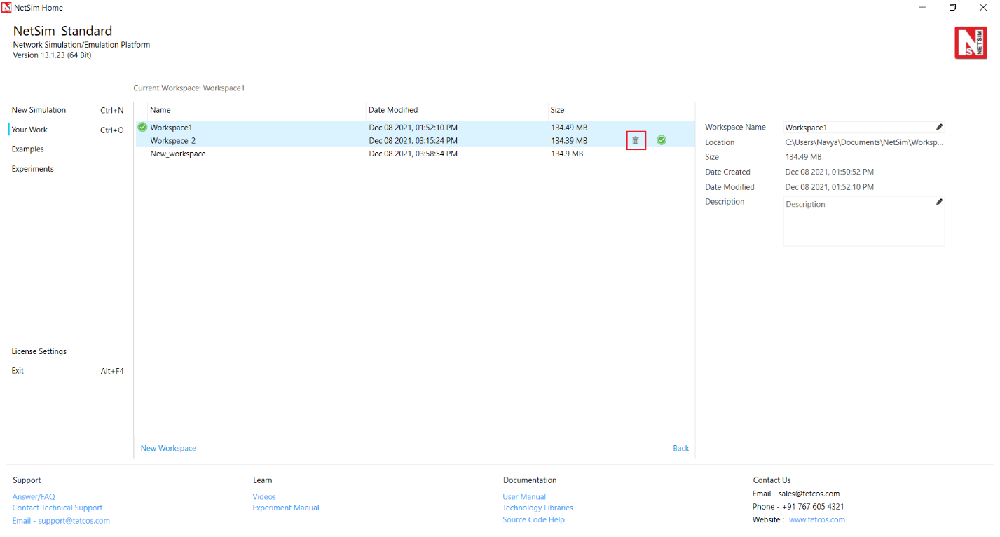


 in
the header of the column you want to filter. In the list of text or
numbers, uncheck the (Select All) box at the top of the list, and then
check the boxes of the items you want to show.
in
the header of the column you want to filter. In the list of text or
numbers, uncheck the (Select All) box at the top of the list, and then
check the boxes of the items you want to show.


 Figure
10‑4: NetSim_utility.h file in IEEE802_11.c file
Figure
10‑4: NetSim_utility.h file in IEEE802_11.c file

 Figure 10‑7: Including the
NetSim_utility.h file in Medium.c file
Figure 10‑7: Including the
NetSim_utility.h file in Medium.c fileFigure 10‑8: Defining a new function matlab_calculate_facingloss() in the Medium.c file


 Figure ‑: Adding
Neighbor and Performing 2-way Event if neighbor is present in Router’s
list.
Figure ‑: Adding
Neighbor and Performing 2-way Event if neighbor is present in Router’s
list.


