Introduction#
NetSim satellite library models end-to-end, full stack, packet level communication between terrestrial nodes and Geostationary satellites. Geo satellites have the unique property of remaining permanently fixed in exactly the same position in the sky as viewed from any fixed location on Earth. This means ground-based antennas do not need to track them but can remain fixed in one direction. These satellites have orbital period that is the same as Earth’s rotation period and are the most common type of communications satellites.
The Satellite MAC layer protocol supported in NetSim is TDMA for forward link and MF-TDMA for return link (based on the DVB S2 standards). The forward link is in the Ku band (12 – 18 GHz) while the return link is in the Ka band (26 – 40 GHz)
The satellite can be thought of as a relay station. It operates on the bent-pipe (transparent star) principle, sending back to Earth what comes in, with only amplification and a shift from uplink to downlink frequency.
In NetSim, the satellite communication network library interfaces with Internetworks library. This means users can connect Satellite gateway and User Terminals to devices such as Routers, Switches Wired nodes, Access point and Wireless nodes etc.

Figure ‑: NetSim GUI showing Satellite User Terminals connected to a server via satellite links
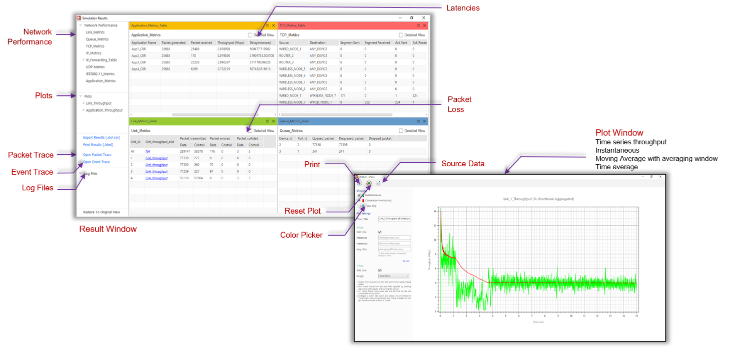
Figure ‑: The Result dashboard and Plot window shown in NetSim after completion of simulation
The PHY layer models include:
-
Channel model: Friis free space path loss with Loo Markov fading model.
-
Modulation: QPSK, 8PSK, 16APSK, 16QAM, 32APSK with appropriate coding rates.
-
Tx, Rx Antenna gains.
-
Antenna gain to noise temperature.
All the choices of transport protocols, and all types of applications in unicast mode can be run.
NetSim’s protocol source C code shipped along with (standard / pro versions) is modular and customizable to help researchers to design and test their own sat-com protocols.
Simulation GUI#
Open NetSim, Go to New Simulation Satellite Comm. Networks

Figure ‑: NetSim Home Screen
Create Scenario#
Satellite Communication Networks palette features various devices like Wired Nodes, L2 Switch, Access Point, Wireless node, UT Router (User Terminal Router), Router, UT Node (User Terminal Node), Satellite Gateway, and Satellite.
Devices specific to NetSim Satellite Comm. Library#
- UT - User Terminal. The user terminals are part of the same communication network as the Satellite Gateway. The User Terminals in NetSim are UT_Node and UT_Router
-
UT Router - User Terminal Router. A UT_Router is used when a separate communication network is required. The typical use case is where there are multiple devices downstream who seek to utilize the sat-com link. The UT Router cannot be a source of any traffic.
-
Satellite Gateway: Each gateway has two interfaces, a satellite interface and multiple wired interfaces. The satellite interface connects via the forward link to the satellite. The wired interface allows for connection to routers via the wired interface. When connected to a satellite, the user terminals mapped to the gateway are part of the same network. Multiple gateways can be configured per satellite, and round-robin scheduling is run (at the Network control center (NCC) which is not displayed in NetSim GUI)
-
Satellite: Since the satellite model is a bent pipe the satellite does not have an IP. Each satellite can be connected to multiple gateways and to multiple User_Terminals. The satellite node cannot be the source of any traffic. The default altitude of the Satellite is 35,768,000 meters, which represents the circular geosynchronous orbit. Multiple satellites can be configured per scenario. However, no interference is modeled when multiple satellite communication occurs simultaneously.
-
Coordinate System: NetSim uses a Geodetic co-ordinate system. The altitude is from Mean Seal level. The geocentric co-ordinate system uses distance from the centre of the earth.

Figure ‑: The devices present in the ribbon in NetSim’s GUI
Placement of devices on the grid environment#
- Add a User Terminal (UT) – Click the User_Terminal > UT_Node icon on the toolbar and place the device in the grid. UT_Node must be connected to Satellite.
-
Add a UT Router – Click the User_Terminal > UT_Router icon on the toolbar and place the device in the grid. UT_Router must be connected to a Node or to a L2_Switch or to a Router or to an Access_Point or Satellite.
-
Add a Satellite – Click the Satellite icon on the toolbar and place the Satellite in the grid. Satellite must be connected to a Satellite_Gateway or to a UT_Node or to a UT_Router.
-
Add a Satellite_Gateway – Click the Satellite_Gateway icon on the toolbar and place the Satellite_Gateway in the grid. Satellite_Gateway must be connected to a Satellite or to a Router.
-
Add a Router – Click the Router icon on the toolbar and place the Router in the grid.
-
Add a Wired Node – Click the Wired_Node icon on the toolbar and place the device in the grid.
-
Add a L2_Switch – Click the L2_Switch icon on the toolbar and place the device in the grid.
-
Add an Access_Point – Click the Access_Point icon on the toolbar and place the Access_Point in the grid.
-
Add a Wireless Node – Click the Wireless Node icon on the toolbar and place the device in the grid.
NOTE: It is recommended not to connect multiple satellite gateways to a single satellite since this can leads to IP address and static route complications
GUI Configuration Parameters#
The SATELLITE parameters can be accessed by right clicking on a Satellite, Satellite Gateway, UT Router or UT and selecting Interface (SATELLITE) Properties Datalink and Physical Layers.
| Satellite Properties | ||||
|---|---|---|---|---|
| Interface (Satellite) – Physical Layer | ||||
| Parameter | Type | Range | Description | |
| G/T (dBk) | Local | 0-100000dBk | Antenna gain-to-noise-temperature is (G/T) where G is the antenna gain in decibels at the receive frequency, and T is the equivalent noise temperature of the receiving system in kelvins. | |
| Tx Power | Local | 0-10000dBW | It is the signal intensity of the transmitter. The higher the power radiated by the transmitter's antenna the greater the reliability of the communications system. | |
| Access Protocol | Fixed | TDMA | TDMA allows a number of clients to access a single radio-frequency channel without interference by allocating unique time slots to each user within each channel, reducing the loss of packets and improving the data rate thereby delivering QoS to the clients. | |
| Fixed | MF-TDMA | Multi-frequency time-division multiple access is a technology for dynamically sharing bandwidth resources in an over-the-air two-way communications network. | ||
| Base Frequency (GHz) | Local | Ku-band: 12-18GHz Ka-band: 26-40GHz |
The “band” in use refers to the radio frequencies used to and from the satellite: Ku-band services uses the 12 - 18 GHz, and Ka-band services uses the 26- 40 GHz segment of the electromagnetic spectrum |
|
| Band | Fixed | KU | Microwave frequency band used for satellite communication and broadcasting, using frequencies in the range of 12 -18 GHz | |
| Fixed | KA | Microwave frequency band used for satellite communication and broadcasting, using frequencies in the range of 26 - 40 GHz | ||
| Rolloff Factor | Local | 0-1 | In NetSim, Symbol Rate = BW / (1+Roll of factor) and Bit Rate = Symbol rate * Modulation order * CodeRate |
|
| Spacing Factor | Local | 0-1 | In NetSim EffectiveBandwidth (Hz) = AllocatedBandwidth (Hz) / ((RollOffFactor + 1.0) * (SpacingFactor + 1.0)); Spacing factor should be in the range of [0,1] |
|
| Carrier Bandwidth (Hz) | Local | 0-1000000 Hz | Bandwidth of the carrier in Hz | |
| Framecount in Superframe | Local | 0-1000000 | Number of frames present in a superframe. | |
| Frame Bandwidth (Hz) | Local | 0-1000000 Hz | Bandwidth of the frame in Hz. | |
| Frame Usage Mode | Local | NORMAL SHORT |
Baseband frame usage modes. | |
| Modulation | Local | QPSK 8PSK 16APSK 16QAM 32APSK |
Modulation is the process of varying one waveform in relation to another waveform. It is used to transfer data over an analog channel. | |
| Coding Rate | Local | 1/3,1/2, 3/5, 2/3, 3/4, 4/5, 5/6, 8/9, 9/10 | It states what portion of the total amount of information that is useful(non-redundant). This code rate typically a fractional number. | |
| Slot Count in Frame | Local | Short Frame: QPSK-90, 8PSK-60, 16APSK/16QAM-45, 32APSK-36 Normal Frame: QPSK-360, 8PSK-240, 16APSK/16QAM-180, 32APSK-144 |
The number of slots per frame. The number of slots per frame is based on modulation and frame type chosen. | |
| Symbol Rate | Local | 0-1000000 | It is ratio of total bandwidth and (1+ Roll of Factor) | |
| Symbol per Slot | Local | 0-1000000 | The number of TDMA symbols within a slot, the default value of symbol per slot is 90. | |
| Pilot Block Size (Symbols) | Local | 0-1000000 symbols | Size of pilot block in symbols | |
| Pilot Block Interval (Slots) | Local | 0-1000000 slots | Interval (in symbols) between Pilot blocks | |
| Pilot Header (Slots) | Local | 0-1000000 slots | The pilot block header size in slots. | |
| Frame Header Length (Bytes) | Local | 0-1000000 bytes | Baseband frame header length in bytes | |
| BER Model | Local | Fixed | BER value is based on the user input. | |
| FILE BASED | File Based is a feature in NetSim with which users can define the BER. Users will have to provide a BER_FILE.txt file as input to NetSim by clicking on the Open file link the Physical Layer-Properties of the device. | |||
| MODEL_BASED | The BER model, calculates the BER via the pathloss model for the particular scenario. | |||
| BER | Local | 0.00000001-1 | This is the rate at which errors occur in the transmission of digital data. | |
| UT Properties | ||||
| Interface (Satellite) – Physical Layer | ||||
| Parameter | Parameter | Parameter | Parameter | |
| Tx Antenna Gain (dB) | Local | 0-1000000dB | A relative measure of an antenna’s ability to direct or concentrate radio frequency energy in a particular direction or pattern at the transmitter side. | |
| Rx Antenna Gain (dB) | Local | 0-1000000dB | A relative measure of an antenna’s ability to receive radio frequency energy in a particular direction or pattern at the receiver side. | |
| Table 2‑1: Satellite, Satellite Gateway, UT Router or UT and selecting Interface (SATELLITE) Properties Datalink and Physical Layers Description | ||||
| Propagation Model | ||||
| Link Properties | ||||
| Parameter | Type | Range | Description | |
| Propagation Medium | Link | Air | Medium of propagation in NetSim would be Air for RF waves. | |
| Channel Characteristics | Fixed | Pathloss and Fading and Shadowing | Path loss and fading and shadowing: In pathloss models, for a fixed distance between source and destination, path loss is same. We get varied path loss for some distance between source and destination in shadowing and fading is variation of the attenuation of a signal with various variables. These variables include time, geographical position, and radio frequency. | |
| Shadowing Model | Fixed | NONE | ||
| Pathloss Model | Link | Friis Free Space | It Used to model the LOS path loss incurred in the channel. the Friis Free space model is restricted to unobstructed clear path between the transmitter and the receiver. | |
| Pathloss Exponent (η) | Fixed | 2 | Path loss exponent indicates the rate at which the path loss increases with distance. The value depends on the specific propagation environment. | |
| Fading Model | Fixed | Markov Loo | Each state of the three-state Markov channel models obeys the Loo distribution with different parameters; while the state transition is modeled as a first-order Markov random process. | |
| Direct Signal Mean (dB) | Link | -∞ to ∞ | Mean value of the direct signal, value can be differentiated according to the state. | |
| Direct Signal Standard Dev (dB) | Link | 0 to ∞ | Standard Deviation of the direct signal value can be differentiated according to the state. | |
| RMS Multipath Power (dB) | Link | -∞ to ∞ | RMS squared multipath power in dB | |
| Number of Direct Signal Oscillators | Link | 0 to ∞ | Number of direct signal oscillator is used for frequency conversion process in superheterodyne receiver. | |
| Number of Multipath Oscillators | Link | 0 to ∞ | Number of multipath oscillators is used to generate higher oscillation frequencies. | |
| Direct Signal Doppler (Hz) | Link | 0 to ∞ | ||
| Multipath Doppler (Hz) | Link | 0 to ∞ | The normalized PSD (its integral in the whole frequency range equals to one) constitutes the PDF for the Doppler frequencies, arising from the different angles of arrival the multipath components have with respect to the receiver’s motion. | |
| Initial Probability | Link | 0 to 1 | An initial probability distribution, defined on S, specifies the starting state. Usually this is done by specifying a particular state as the starting state. | |
Table ‑: Propagation Model/Wireless Link Properties Description
Mapping of User_Terminal (UT_Note / UT_Router) to Satellite_Gateway#
Each satellite can be connected to multiple Satellite_Gateways and to Multiple User_Terminals. The following screen shot shows how to map the User_Terminal to Satellite_Gateway as shown Figure 2‑3.

Figure ‑: Mapping of User_Terminal (UT_Note / UT_Router) to Satellite_Gateway
In order to Map User_Terminal (UT_Node / UT_Router) to Satellite_Gateway right click go to the properties of UT_Node/UT_Router INTERFACE1_(SATELLITE) DATALINK_LAYER Gateway user can map the Satellite_Gateway with UT_Node / UT_Router accordingly.
Additionally, in the UT_Router/UT_Node -> Interface_Satellite the default gateway IP should be set as the IP of the connected Satellite_Gateway.
Incorrect mapping of the Satellite_Gateway and/or the default_Gateway IP address, in the properties of the UT_Node / UT_Router could lead application crash or NIL application throughputs.
Configuring Static Routes#
After mapping the UT_Router/UT_Node to a Satellite_Gateway, static routes need to be configured in the devices to forward traffic. Let us consider the following network scenario as shown Figure 2‑4.

Figure ‑: Network Topology in this experiment
In this network scenario, for UDP traffic to be sent from UT_Node_2 to UT_Node_3, static routes need to be set in UT_Node_2 and in the Satellite_Gateway_4.
If TCP traffic needs to be sent from UT_Node_2 to UT_Node_3, then static routes need to be set in UT_Node_3 as well. This is essential for connection establishment and sending acknowledgements.
Refer the featured example on Configuring applications from UT Node to UT Node for detailed information on static route configuration.
Model Features#
TDMA Forward Link and MF TDMA Return Link#

Figure ‑: Forward and Return links. The Network Control Centre (NCC) is not displayed in NetSim and is assumed to be part of every satellite
In NetSim, a Forward link is defined as the direction from Satellite Gateway to Satellite to UT_Node / UT_Router. A Return link is defined as the direction from the UT_Node / UT_Router to Satellite to the Satellite Gateway.
The protocol operating in the Forward link is Time Division Multiple Access (TDMA). The protocol operating in the Return link is Multi Frequency Time Devision Multiple Access (MF-TDMA).
Both the Forward link and Return link transmissions in NetSim are modeled as Layer-2 transmissions. The framing is as explained in the subsequent paragraph.
Each Super Frame is composed of a number of Frames. This is taken as a user input, given by the attribute Framecount_in_SuperFrame available in Satellite -> Interface_Satellite -> Physical_Layer properties. The frames in turn are composed of carriers (in frequency) and slots (in symbols). The number of carriers would be
$$Number\ of\ Carriers = \frac{Frame\ Bandwidth\ (Hz)}{Carrier\ Bandwidth\ (Hz)}$$
The number of slots per frame is determined by the modulation scheme chosen by the user.
Modulation and coding schemes supported#
-
QPSK with coding rates 1/3, 1/2, 3/5, 2/3, 3/4, 4/5, 5/6, 8/9, 9/10
-
8PSK with coding rates 3/5, 2/3, 3/4, 5/6, 8/9, 9/10
-
16APSK with coding rates 2/3, 3/4, 4/5, 5/6, 8/9, 9/10
-
16QAM with coding rates 3/4, 5/6
-
32APSK with coding rates 3/4, 4/5, 5/6, 8/9
Physical layer framing for forward and return links#

Figure ‑: Format of a “Physical Layer Frame” PLFRAME
\[\mathbf{\eta}_{\mathbf{ldpc}}\mathbf{= 64800\ }\] \[\mathbf{(normal\ frame)}\] |
\[\mathbf{l = 16200\ }\] \[\mathbf{(short\ frame)}\] |
|||
|---|---|---|---|---|
| \[\mathbf{\eta}_{\mathbf{MOD}}\mathbf{\ (bits/Hz)}\] | \[S\] | \[\eta\ \%\ no - pilot\] | \[S\] | \[\eta\ \%\ no - pilot\] |
| 2 | 360 | 99.72 | 90 | 98.90 |
| 3 | 240 | 99.59 | 60 | 98.36 |
| 4 | 180 | 99.45 | 45 | 97.83 |
| 5 | 144 | 99.31 | 36 | 97.30 |
Table ‑: S = number of SLOTs per FRAME (number of symbols per slot is 90)
The normal frame and short frame setting can be done using the Frame_Usage_Mode parameter in the GUI as shown Figure 3‑3.
Changing the Modulation scheme in UI would change the value of S (Slot_count_in_frame)

Figure ‑: Satelittle > Physical layer properties window
Default NetSim GUI settings
-
Symbols per slot: 90
-
Pilot Block size (symbols): 36
-
Pilot block interval (slots): 16
-
PL header size (slots): 1
-
Frame header size (In bytes): 10 (per ETSI EN 302 307 V1.3.1)
-
Frame Type: Normal (Options are normal or short)
Satellite PHY: Data Rate#
Given below is the data rate calculation methodology for both forward and return links. The parameter values used are the default values in NetSim GUI.
$$Symbol\ Rate = \frac{BW}{\left( 1 + (Roll\ of\ factor) \right)}$$
Bit Rate = Symbol rate × Modulation order × CodeRate
Bandwidth (Hz) = Frame_Bandwidth (Hz) = 106 Hz
$$Central\ Frequency\ (Hz) = Base\ Frequency\ (Hz) + \frac{Bandwidth\ (Hz)}{2.0}$$
$$Central\ Frequency\ (Hz) = 26 \times 10^{9} + \ \frac{10^{6}}{2} = 26000500000\ Hz$$
$$Effective\ Bandwidth\ (Hz) = \frac{\ Carrier\ Bandwidth\ (Hz)}{(RollOfFactor + 1.0) \times (SpacingFactor + 1.0)}$$
$$Effective\ Bandwidth\ (Hz) = \frac{10^{6}}{(1.0 + 1.0) \times (1.0 + 1.0)} = 25 \times 10^{4}\ Hz$$
Symbol Rate = Effective Bandwidth (Hz) = 25 × 104Hz
Modulation Bits = 2
The number of Modulation Bits depends on the modulation scheme per the table below:
| Modulation | Modulation bits |
|---|---|
| QPSK | 2 |
| 8PSK | 3 |
| 16APSK/16QAM | 4 |
| 32APSK | 5 |
Table ‑: Modulation bits for different modulation
Slots = Slot Count in Frame + Pilot Header (slots) = 360 + 1 = 361
Data Symbols = Slots × Symbol per Slot = 361 × 90 = 32490
$$Pilot\ Slot = \frac{Slots}{Pilot\ Block\ Interval} = \frac{361}{16} = 22$$
Pilot Symbol = Pilot Slot × Pilot block Size (symbols) = 22 × 36 = 792 Symbols
Total Symbol = Pilot Symbol + Data Symbols = 792 + 32490 = 33282
$$Frame\ length = \frac{Total\ Symbol}{Symbol\ Rate} \times 1000000 = \frac{33282}{250000} \times 1000000 = 133128\ \mu s$$
$$Pilot\ Block\ Length = \frac{Pilot\ block\ Size\ }{Symbol\ Rate} \times 1000000 = \frac{36}{250000} \times 1000000 = 144\ \mu s$$
$$Slot\ Length = \frac{Symbol\ per\ Slot}{Symbol\ Rate} \times 1000000 = \frac{90}{250000} \times 1000000 = 360\ \mu s$$
SuperFrame Duration = Frame length × Frames per SuperFrame = 133128 × 10 = 1331280 μs
$$Bits\ per\ Slot = Symbol\ per\ slot\ \times Modulation\ Bits \times Coding\ Rate = 90 \times 2 \times \frac{1}{2} = 90$$
Bits per Frame = Bits per Slot× Slot Count in Frame = 90 × 360 = 32400
$$Data\ Rate = \frac{Bits\ per\ Slot}{Slot\ Length} = \frac{90\ bits}{360\ \mu s} = 0.25 \times 10^{6}\ bits/sec = 0.25\ Mbps$$
Analytical throughput estimation#
Let us an example in which the Packet Size (App layer) is 1460B which translates to 1488B at the PHY layer after addition of overheads, with QPSK modulation and $\frac{1}{3}$ coding rate. For this modulation and coding rate the raw PhyRate of the channel is 162249 bps using the formulas given in 3.4. The analytical throughput estimate for such a scenario would be:
$$PacketTransmissionTime = \frac{PacketSize(at\ PHY) \times 8}{PhyRate(bps)} = \frac{1488 \times 8}{162249} = 0.0733687s = 73368.7\mu s$$
$$PacketsPerFrame = \lfloor\frac{FrameTime}{PacketTransmissionTime}\rfloor = \lfloor\frac{133128}{73368.7}\rfloor = \lfloor 1.81\rfloor = 1\ $$
PacketsPerFrame is the number of packets that can be packed in a frame, and hence the greatest integer or floor function is used.
BytesPerFrame = PacketsPerFrame × PacketSize(B) = 1488 × 1 = 1488
$$NumberOfFramesPerSecond = \frac{1}{Frame\ Duration(s)} = \frac{1}{0.133128} = 7.51$$
PhyThroughput = NumberOfFramesPerSecond × (BytesPerFrame×8) = 7.51 × (1488×8) = 89399.04 bps = 0.089 Mbps
$$ApplicationThroughput = \frac{1460}{1488} \times PhyThroughput = 0.087\ Mbps$$
PHY rate for various modulations and coding rates#
| Modulation | Modulation bits | Slot Count in a frame | Coding Rate | PHY Rate (Mbps) |
|---|---|---|---|---|
| QPSK | 2 | 360 | 1/3 | 0.167 |
| 1/2 | 0.250 | |||
| 3/5 | 0.300 | |||
| 2/3 | 0.333 | |||
| 3/4 | 0.375 | |||
| 4/5 | 0.400 | |||
| 5/6 | 0.417 | |||
| 8/9 | 0.444 | |||
| 9/10 | 0.450 | |||
| 8PSK | 3 | 240 | 3/5 | 0.450 |
| 2/3 | 0.500 | |||
| 3/4 | 0.561 | |||
| 5/6 | 0.625 | |||
| 8/9 | 0.667 | |||
| 9/10 | 0.675 | |||
| 16APSK | 4 | 180 | 2/3 | 0.667 |
| 3/4 | 0.750 | |||
| 4/5 | 0.800 | |||
| 5/6 | 0.833 | |||
| 8/9 | 0.889 | |||
| 9/10 | 0.900 | |||
| 16QAM | 4 | 180 | 3/4 | 0.750 |
| 5/6 | 0.833 | |||
| 32APSK | 5 | 144 | 3/4 | 0.936 |
| 4/5 | 1.000 | |||
| 5/6 | 1.042 | |||
| 8/9 | 1.111 |
Table ‑: List of support modulation schemes and coding rates, and their respective PHY Rates
Satellite PHY: Land Satellite Channel Model#
Propagation#
The distance between the ground nodes and the satellite determines the propagation delay and path loss of the radio signal. The distance is computed based on the cartesian distance between the ground nodes and the satellite. NetSim computes the propagation delay of the radio signal traveling from the source node to the destination node at the speed of light. The propagation model calculates the weakening of the radio signal as it propagates from the source node per the pathloss and fading model.
Pathloss Model – Friis Free Space Propagation#
The free space propagation model is used to predict received signal strength when the transmitter and receiver have a clear, unobstructed line-of-sight path between them. Satellite communication systems and microwave line-of-sight radio links typically undergo free space propagation. The free space power received by a receiver antenna which is separated from a radiating transmitter antenna by distance d, is given by the Friis free space equation.
$$\ P_{r}\ = \ P_{t} + \ G_{t} + \ G_{r} + \ 20\log_{10}{\left( \frac{\lambda}{(4*\pi*do)} \right)\ }\ + \ \left( 10 \times 2 \times \log_{10}\left( \frac{do}{d} \right) \right)$$
where Ptis the transmitted power.
Pr is the received power.
Gt is the transmitter antenna gain.
Gr is the receiver antenna gain.
d is the T-R separation distance in meters.
λ is the wavelength in meters.
Fading model#
NetSim uses a 3 state (state 1, state 2 and state 3) Markov model to simulate fading.
The conditional probabilities of state sn + 1 given the state snare described by state transition probabilities pij
Where S1, S2, S3 denotes respective channel state, Pij is the probability the Markov process goes from state i to state j.

Figure ‑: Switching of three-state Markov process
The switching among each state is described by a transition metrix P, which is
p11 p12 p13
P= p21 p22 p23
p31 p32 p33
Each state of the three-states of the Markov model obeys the Loo distribution with different parameters, while the state transition is modeled as a first-order Markov random process.
The Loo distribution considers the received signal as a sum of two signal components. A log-normally distributed direct signal expresses the slow fading component corresponding to varying shadowing conditions of the direct signal. A Rice distribution characterizes the fast-fading component due to multipath effects.
The Loo parameter triplet consists of the mean, the standard deviation for the log-normally distributed direct signal, and the average multipath power.
N(μ, σ2) + R
Depending on the current state interval and on the environment of the terminal, a new random Loo parameter triplet is generated. The output of the channel model is a time-series of the received signal in form of a complex envelope.
And finally, the model computes the Loo distributed time-series including Doppler shaping for every new state interval, which is the output of the proposed LMS channel model.

Figure ‑: The Satellite LMS channel Model
SNR - BER Calculation#
$${SNR\ (dBm) = \ log}_{10}\left( \frac{Received\ power\ (in\ mW)}{\ Thermal\ Noise\ (in\ mW)} \right)$$
The SNR is calculated separately for each ‘hop’ of each link. This means the calculation is done from Gateway to Satellite and then separately again from Satellite to UT, and vice versa.
Noise = kB T B where kBis the Boltzman’s constant, B is the carrier bandwidth and T is the temperature calculated per user input of $\frac{G}{T}(dBK)\ $in NetSim UI.
NetSim provides three options for BER.
-
Model Based: The BER is then calculated for each link based on the SNR. Please see Propagation-Models.pdf document for detailed information on BER calculation.
-
Fixed: the BER value can be input in the GUI. If this option is chosen, the SNR (derived from propagation model) is not used.
-
File Based: SNR – BER table should be provided in a file per the format given below. This table should be in increasing order of SNR. The SNR is calculated by NetSim from the RF propagation model. For this SNR, the appropriate BER is selected from this table. BER is 1.0 for any SNR value below SNR1, and BER is 0.0 for any SNR greater than SNRn.
SNR1, BER1
SNR2, BER2
…
SNRn, BERn
Results#
Please see NetSim User manual, Results and Analysis section.
Satellite Log File#
NetSim Satellite Log file records UT Satellite association, calculated superframe, frame, slot, bandwidth, etc.,. This log can be enabled/disabled by going to Logs option and checking/unchecking the DTDMA Radio Measurements Log option under the Network Logs section as shown below:

Figure ‑: Enabling Satellite Log file
A log file specific to satellite communication, is generated post simulation as shown in screen shot below,

Figure ‑: Result Window
On opening it would look like the image below

Figure ‑: NetSim Satellite communication log file
This file logs details such as
-
UE – Satellite Gateway association
-
Calculated Super frame, frame, slot, bandwidth, carrier count etc. for each satellite.
-
Frame by frame transmissions with time stamps
Enable Propagation log#
NetSim Satellite Log file records UT Satellite association, calculated superframe, frame, slot, bandwidth, etc,. This log can be enabled/disabled by going to Logs option and checking/unchecking the DTDMA Radio Measurements Log option under the Network Logs section as shown below:

Figure ‑: Enabling Satellite Log file
Additional Satellite Propagation log files will be available under the Log Files menu in the left panel of the Results Window as shown below:

Figure ‑: Result Window
Users can see pathloss, fading-loss, noise, and SNR values in the Log files for each forward and return link.

Figure ‑: Propagation log file
Omitted Features#
-
Regenerative transponder where the signal is demodulated, decoded, re-encoded and modulated aboard the satellite.
-
Impact of Rain/Weather on signal propagation
-
Forward Error Coding in Layer 2
-
IPv6 Addressing
-
No support for LEO, MEO
Featured Examples#
Bandwidth variation through MCS configuration #
Open NetSim, Select Examples ->Satellite Communication -> Bandwidth variation through MCS configuration then click on the tile in the middle panel to load the example as shown in Figure 4‑1.

Figure ‑: List of scenarios for the example of Bandwidth variation through MCS configuration
The following network diagram illustrates, what the NetSim UI displays when you open the example configuration file as shown Figure 4‑2.

Figure ‑: Network set up for studying the Bandwidth variation through MCS configuration
Settings done in example config file:
- Set the following property as shown in below given table:
| Satellite Properties -> Interface (Satellite) -> Physical Layer-> Forward | |
|---|---|
| BER_Model | Fixed |
| BER | 0.00000001 |
Table ‑: Satellite Properties > Interface (Satellite) > Physical Layer > Forward
- Set the following property as shown in below given table:
| UT_Router Properties -> Interface (Satellite) -> DataLink Layer | |
|---|---|
| Gateway | Sat_Gateway_3 |
Table ‑: UT_Router Properties > Interface (Satellite) > DataLink Layer
- Go to Router_4 properties -> Network_Layer ->Enable - Static IP Route ->Configure Static Route IP

Figure ‑: Router Network layer properties window
- Set the properties in Static Route IP window as per the screenshot below and click on Add. Click on OK.

Figure ‑: Configuring Static route window for router
-
Go to Sat_Gateway_3 properties -> Network_Layer ->Enable - Static IP Route ->Configure Static Route IP Set the properties in Static Route IP window as per the screenshot below and click on Add. Click on OK.

Figure ‑: Configuring Static route window for Sat_Gateway_3
-
Go to UT_Router_2 properties -> Network_Layer -> Enable - Static IP Route -> Configure Static Route IP Set the properties in Static Route IP window as per the screenshot below and click on Add. Click on OK.

Figure ‑: Configuring Static route window for UT_Router_2
-
CBR application source id as 6 and destination id as 5 with packet size as 1460Bytes and Inter_Arrival_time as 467μs (Generation Rate=25Mbps). Transport Protocol is set to UDP.
-
Change the Satellite Properties Interface (Satellite) Physical_Layer Forward Modulation and respective coding rates as sshown in below Table 4‑3 but for return link is fixed Modulation-> 32APSK and Coding Rate ->3/4.
-
In NetSim GUI Plots are Enabled. Run simulation for 10 seconds and observe the result.
NOTE: Satellite properties in the physical layer changes done only for the forward and Return layer properties.
Result: Observe the application throughput as we change the modulation scheme (Satellite Properties Interface (Satellite) Physical_Layer Forward Modulation) and respective coding rates (Satellite Properties Interface (Satellite) Physical_Layer Forward Coding_Rate).
| Modulation | Coding_Rate | Throughput (Mbps) |
|---|---|---|
| QPSK | 1/3 | 0.084 |
| 9/10 | 0.336 | |
| 8PSK | 3/5 | 0.380 |
| 9/10 | 0.507 | |
| 16APSK | 2/3 | 0.507 |
| 9/10 | 0.677 | |
| 16QAM | 3/4 | 0.676 |
| 5/6 | 0.675 | |
| 32APSK | 3/4 | 0.846 |
| 8/9 | 0.843 |
Table ‑: Compare the different Modulation Scheme and Coding Rate vs. Througput
Configuring applications from UT Node to UT Node #
Open NetSim, Select Examples ->Satellite Communication -> UT to UT Communication then click on the tile in the middle panel to load the example as shown in below screenshot

Figure ‑: List of scenarios for the example of UT to UT Communication
The following network diagram illustrates, what the NetSim UI displays when you open the example configuration file as shown Figure 4‑8.

Figure ‑: Network set up for studying the UT-to-UT Communication
Settings done in example config file
- Set the following property as shown in below given table:
| UT_Node Properties -> Interface (Satellite) -> DataLink Layer | |
|---|---|
| Gateway | Sat_Gateway_4 |
Table ‑: UT_Node Properties > Interface (Satellite) > DataLink Layer
- Go to UT_Node_2 properties -> Network_Layer -> Enable - Static IP Route ->Configure Static Route IP.

Figure ‑: Network layer properties window for UT_Node_2
- Set the properties in Static Route IP window as per the screenshot below and click on Add. Click on OK.

Figure ‑: Configure static route for UT_Node_2
- Go to Sat_Gateway_4 properties -> Network_Layer -> Enable - Static IP Route ->Configure Static Route IP

Figure ‑: Network layer properties window for Sat_Gateway_4
- Set the properties in Static Route IP window as per the screenshot below and click on Add. Click on OK.

Figure ‑: Configure static route for Satellite_Gateway_4
-
Set Application Properties are default (Packet Size: 1460, Inter Arrival Time: 20000 µs)
-
Set Transport Protocol to UDP
-
Enable Packet Trace, Event Trace and Plots.
-
Run simulation for 100 seconds and observe the result.
Result: Go to the result window and open packet trace/ Animation window user can observe the packet flow from UT node (source) Satellite Sat gateway Satellite UT node (destination)

Figure ‑: Animation Window

Figure ‑: Packet Trace
Reference Documents#
-
ETSI EN 301 545-2 V1.2.1 (2014-04). Digital Video Broadcasting > (DVB); Second Generation DVB. Interactive Satellite System > (DVB-RCS2); Part 2: Lower Layers for Satellite standard
-
ETSI EN 302 307 V1.2.1 (2009-08). Digital Video Broadcasting (DVB); > Second generation framing structure, channel coding and modulation > systems for Broadcasting, Interactive Services, News Gathering and > other broadband satellite applications (DVB-S2)
-
Lu Lu, Daoxing Guo, Aijun Liu and Maoqiang Yang (2012). Analysis of > Channel Model for GEO Satellite Mobile Communication System. In > National Conference on Information Technology and Computer Science > (CITCS 2012)
-
Chun Loo (1985). A Statistical Model for a Land Mobile Satellite > Link. IEEE Transactions on Vehicular Technology, 1985, 34(8): > 122-127.