Radio Propagation
Pathloss, Shadowing and Fading (Level 1)
Part 1: Pathloss and Shadowing
Log-distance pathloss
Path loss is the reduction in power density of an electromagnetic wave as it propagates through space. Path loss is a positive quantity measured in dB and is defined as the difference (in dB) between the transmitted power and the received power and may or may not include the effect of antenna gains.
Both theoretical and measurement-based propagation models indicate that average received signal power decreases logarithmically with distance whether in outdoor or in indoor ratio channels. The average large-scale pathloss for an arbitrary transmitter-receiver separation is expressed as a function of distance by using the pathloss exponent \(\eta\), which indicates the rate at which the pathloss increases with distance [4]. Therefore pathloss \(PL(d) \propto \left( \frac{d}{d_{0}} \right)^{\eta}\).
The general formula (when written in dB scale) by which received power is calculated when using the log-distance model and including the effect of antenna gains is
\[P_{r} = P_{t} + G_{t} + G_{r} + 20 \cdot \log_{10}\left( \frac{\lambda}{\left( 4 \cdot \pi \cdot d_{0} \right)} \right) + \ \left( 10 \cdot \eta \cdot \log_{10}\left( \frac{d_{0}}{d} \right) \right)\]
Where,
\(P_{r}\) is the received power,
\(P_{t}\) is the transmit power,
\(G_{t}\) is the transmitter antenna gain, and \(G_{r}\) is the receiver antenna gain.
𝑑 is the distance between the transmitter and receiver.
𝑑0 is the reference distance, and the model is applicable only for \(d > d_{0}\)
𝜆 is the wavelength and is equal to \(\frac{c}{f}\) where 𝑐 is the speed of light and 𝑓 is the frequency in \(Hz\)
\(\eta\) is the path loss exponent, whose value is normally in the range of 2 to 5,
Define \(PL_{d0},\)the path loss at reference distance as \(PL_{do} = \ 20 \cdot \log_{10}\left( \frac{4 \cdot \pi \cdot d_{0}}{\lambda} \right).\) Now, when the antenna gains at the transmitter and receiver is unity, i.e., when \(G_{t} = G_{r} = 0\ dB\), the general pathloss formula can be re-written as
\[P_{r} = P_{t} - \underset{Pathloss}{\overset{\left( PL_{d0} + 10 \cdot \eta \cdot \log_{10}(d) \right)}{︸}}\]
which shows us that (in the dB scale) the received power is the transmitted power minus the pathloss.
Log Normal Shadowing
With pathloss models the predicted path loss between a transmitter and a receiver is constant for a given distance. However, different types of terrain and clutter may exist in the transmitter-receiver path. Therefore, the path losses may be vastly different than the average value predicted in (1), for two different locations having the same transmitter-receiver separation distance. Some paths undergo more loss while others are less obstructed and may have higher received signal strength. The variation of path loss with respect to the mean path loss values predicted by the propagation models, depending on the type of environment is called shadowing. Shadowing is also termed shadow-fading or slow fading.
Models for path loss and shadowing can be superimposed to capture power fall off versus distance along with the random attenuation about this average path loss from shadowing. Empirical studies have shown that this randomness is captured well by a second factor, \(S\), of the form\(\ 10^{- \frac{\chi}{10}}\) with \(\chi\\)being a Gaussian random variable with mean \(0\) and variance \(\sigma^{2}\). This is called the shadowing component of the attenuation, and, since \({10 \cdot log}_{10}{(S)}\\)has a Gaussian (or normal) distribution, it is called log-normal shadowing [5]. In the combined model the total loss in dB scale is given by
\[P_{r} = P_{t} - \underset{Pathloss}{\overset{\left( PL_{d0} + 10 \cdot \eta \cdot \log_{10}(d) \right)}{︸}}\ - \underset{shadowing}{\overset{\chi}{︸}}\]
Where \(\chi\) is a zero-mean Gaussian distributed random variable (in dB) with standard deviation \(\sigma\) (in dB). In NetSim, the default value for \(\sigma\) 𝑖𝑠 \(5\ dB\), and the range of \(\sigma\) (in dB) is \(5\ \leq \ \sigma\ \leq \ 12\).
Network Setup
Pathloss
Step 1: Open NetSim and click on Mobile Ad hoc Network.
Step 2: Create a scenario with 2 wireless nodes.
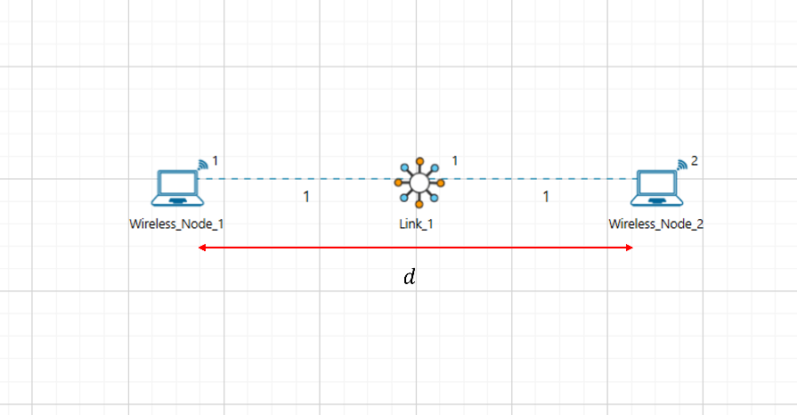
Figure 7‑1: A Network consists of 2 Wireless Nodes. Wireless Node 1 and Wireless Node 2 separated by distance \(\mathbf{d}\) in meters. The values of \(d\) are provided in Table 7‑4.
Step 3: Go to the Properties of Wireless Node 1 🡪 Position Layer 🡪 Mobility Layer 🡪 Mobility Model set to No Mobility.
Step 4: Go to the Properties of Wireless Node 1 🡪 Network Layer 🡪 Enable the static route.
Step 5: Configure static routing in Wireless Node 1 as shown in below Figure 7‑2

Figure 7‑2: Configure Static Routing in Wireless Node 1 via GUI
Step 6: Configure the Wireless link properties as per Table 7‑1.
| Link_1 Properties | |
|---|---|
| Channel Characteristics | Pathloss |
| Pathloss Model | Log distance |
| Pathloss Exponent (\(\mathbf{\eta}\)) | 3 |
Table 7‑1: Wireless Link Properties.
Step 7: To configure the Application Traffic, Go to Set Traffic Tab and set the properties as below in Table 7‑2.
| Application Properties | |
|---|---|
| Application Method | Unicast |
| Application Type | CBR |
| Source ID | 1 |
| Destination ID | 2 |
| Start Time (s) | 5 |
| Packet Size (Bytes) | 500 |
| Inter Arrival Time \(\mathbf{(ms)}\) | 20 |
Step 8: Enable the IEEE 802.11 Radio Measurements Log in NetSim GUI from Configure Reports Tab 🡪 Logs Section as shown in Figure 7‑3.
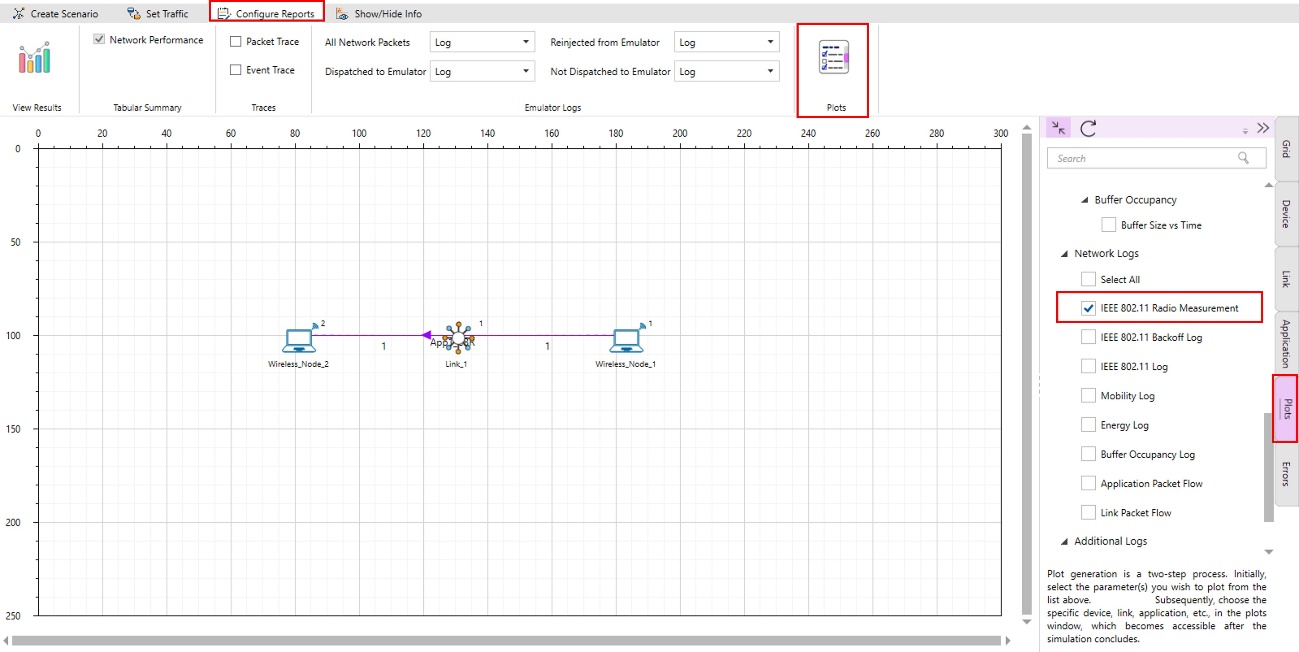
Figure 7‑3: Enabling Radio Measurement Log from GUI
Step 9: Run the simulation for 10 seconds and for each simulation use different seed values.

Figure 7‑4: Run simulation window shown with the seed values.
Step 10: For each simulation vary the distance between the Transmitter that is Wireless Node 1 and Receiver that is Wireless Node 2 as 1, 2, 5, 10, 20, 50, 100, 200 (in meters).
Step 11: Note Down the Pathloss (dB), Receiver Power (dBm) from Radio Measurement log file present under log section in result dashboard.
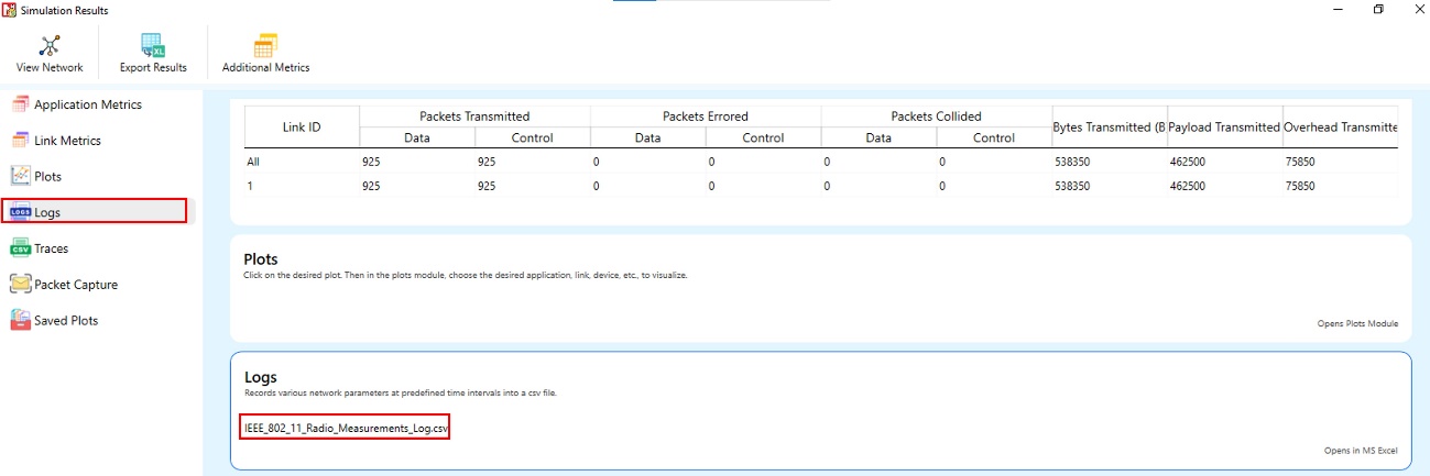
Figure 7‑5: Radio Measurement Log under Logs section in Result Dashboard.
Pathloss and Shadowing
Consider Previous Scenario.
Step 1: Configure the Wireless link properties as per Table 7‑3.
| Link_1 Properties | |
|---|---|
| Channel Characteristics | Pathloss and Shadowing |
| Pathloss Model | Log distance |
| Pathloss Exponent \(\left( \mathbf{\eta} \right)\) | 3 |
| Shadowing Model | Log normal |
| Standard Deviation (dB) | 5 |
Table 7‑3: Wireless Link Properties
Step 2: Run the simulation for 10 seconds and for each simulation use different seed values.
Step 3: For each simulation vary the distance between the Transmitter that is Wireless Node 1 and Receiver that is Wireless Node 2 as 1, 2, 5, 10, 20, 50, 100, 200 (in meters).
Step 4: Note Down the Pathloss (dB), Receiver Power (dBm), Shadowing Loss (dB) and Total Loss (dB) from Radio Measurement log file present under log section in result dashboard.
Results and Discussion
Pathloss
| Distance (m) | RNG Seed 1 |
RNG Seed 2 |
TX Power (dBm) | Path Loss (dB) | RX Power (dBm) |
|---|---|---|---|---|---|
| 1 | 1 | 2 | 20 | 40.09 | -20.09 |
| 2 | 1 | 2 | 20 | 49.12 | -29.12 |
| 5 | 1 | 2 | 20 | 61.06 | -41.06 |
| 10 | 1 | 2 | 20 | 70.09 | -50.09 |
| 20 | 1 | 2 | 20 | 79.12 | -59.12 |
| 50 | 1 | 2 | 20 | 91.06 | -71.06 |
| 100 | 1 | 2 | 20 | 100.09 | -80.09 |
| 200 | 1 | 2 | 20 | 109.12 | -89.12 |
Pathloss and Shadowing
| Distance, \(\mathbf{d}\)(m) | RNG Seed 1 |
RNG Seed 2 |
TX Power (dBm) | Path Loss (dB) | Shadowing Loss (dB) | Total Loss (dB) | RX Power (dBm) |
|---|---|---|---|---|---|---|---|
| 1 | 1 | 2 | 20 | 40.09 | -1.44 | 38.64 | -18.64 |
| 2 | 2 | 3 | 20 | 49.12 | -1.44 | 47.67 | -27.67 |
| 5 | 3 | 4 | 20 | 61.06 | -1.44 | 59.61 | -39.61 |
| 10 | 4 | 5 | 20 | 70.09 | -1.44 | 68.64 | -48.64 |
| 20 | 5 | 6 | 20 | 79.12 | -1.44 | 77.67 | -57.67 |
| 50 | 6 | 7 | 20 | 91.06 | -1.44 | 89.61 | -69.61 |
| 100 | 7 | 8 | 20 | 100.09 | -1.44 | 98.64 | -78.64 |
| 200 | 8 | 9 | 20 | 109.12 | -1.44 | 107.67 | -87.67 |
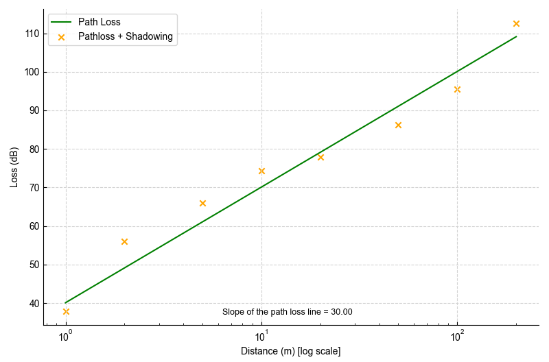
Figure 7‑6: Simulation results of Loss (dB) vs. Distance (m) for Pathloss and for Pathloss with shadowing. The X-axis is a log scale. We can also easily calculate that the slope of the pathloss (green) line is 30 which is the value of \(10 \times \eta\).
On comparing Table 7‑4 and Table 7‑5, we can observe identical pathloss values at equal distances. This shows that the pathloss is deterministic, showing no dependency on the seed used in the random number generator. Recall that \(PathLoss = PL_{d0} + 10 \cdot \eta \cdot \log_{10}(d),\) implying that pathloss plots as a linear line against the logarithm of distance. This is exactly what we observe in the above figure. Furthermore, the slope of this pathloss line turns out to be 30 which is the value of \(10 \times \eta\)configured in the simulation. Both of the above observations are consistent with the log-distance pathloss model. On the other hand, the shadowing loss behaves as a random variable.
Let us theoretically calculate the value of pathloss at a distance of 100m. We know that \(\lambda = \frac{c}{f}\), where \(c,\)the speed of light is taken as \(3 \cdot 10^{8}\ ms^{- 1}\) and the frequency, \(f\) is \(2.412\)GHz.
\[PL(100m) = \ 20 \cdot \log_{10}\left( \frac{4 \cdot \pi \cdot 1}{\left( \left( \frac{3 \cdot 10^{8}}{2.412 \cdot 10^{9}}\ \right) \right)} \right) + \ 10 \cdot \eta \cdot log(100)\]
\[PL(100m) = \ 40.09 + 60 = 100.09\ dB\]
This agrees with the result shown in Table 7‑5.
Part 2: Rayleigh Fading
Introduction
Small-scale fading or simply fading, is used to describe the rapid fluctuation of the amplitude of a radio signal over a short period of time. Fading is caused by interference between two or more versions of the transmitted signal which arrive at the receiver at slightly different times. These waves called multipath waves, combine at the receiver antenna to give a resultant signal which can vary widely in amplitude and phase depending on the distribution of the intensity and relative propagation time of the waves. [4]
Rayleigh fading is widely used to model rapid fluctuations in signal strength due to multipath propagation in wireless networks. In part 1, we saw the impact of two terms pathloss (PL) and shadowing (S) in signal attenuation. The third factor, Rayleigh fading, denoted as \(R^{2}\) has a probability density function (PDF) given by
\[f(x) = \frac{x}{\sigma^{2}}e^{- \left( \frac{x^{2}}{2 \cdot \sigma^{2}} \right)}\]
The distribution of the amplitude attenuation is Rayleigh; hence this is also called Rayleigh fading.
Network Setup
Pathloss
Step 1: Open NetSim and click on Mobile ad hoc Network.
Step 2: Create a scenario with 2 wireless nodes at 100m from each other.

Figure 7‑7: A Network consists of 2 Wireless Nodes. Wireless Node 1 and Wireless Node 2 separated by distance \(\mathbf{100\ m}\).
Step 3: Go to the Properties of Wireless Node 1 🡪 Position Layer 🡪 Mobility Layer 🡪 Mobility Model set to No Mobility.
Step 4: Go to the Properties of Wireless Node 1 🡪 Network Layer 🡪 Enable the static route.
Step 5: Configure static routing in Wireless Node 1 as shown in below figure.

Figure 7‑8: Configure Static Routing in GUI
Step 6: Configure the Wireless link properties as per Table 7‑6.
| Link 1 Properties | |
|---|---|
| Channel Characteristics | Pathloss |
| Pathloss Model | Log distance |
| Pathloss Exponent (\(\mathbf{\eta}\)) | 3 |
Table 7‑6: Wireless Link Properties
Step 7: To configure the Application Traffic, Go to Set Traffic Tab and set the properties as below Table 7‑7.
| Application Properties | |
|---|---|
| Application Method | Unicast |
| Application Type | CBR |
| Source ID | 1 |
| Destination ID | 2 |
| Start Time (s) | 0 |
| Packet Size (Bytes) | 1460 |
| Inter Arrival Time \(\mathbf{(\mu s)}\) | 100000 |
Table 7‑7: Application Properties
Step 8: Enable the IEEE 802.11 Radio Measurements Log in NetSim GUI from Configure Reports Tab 🡪 Logs Section.
Step 9: Run the simulation for 5 seconds.
Step 10: In the Radio Measurement log file present under log section of the result dashboard, filter packet type to CBR and then note down the Time (\(\mu s)\), Pathloss (dB) and Total Loss(dB).
Pathloss and Fading
Consider the previous scenario.
Step 1: Configure the Wireless link properties as per Table 7‑8.
| Link_1 Properties | |
|---|---|
| Channel Characteristics | Pathloss and Fading and Shadowing |
| Pathloss Model | Log distance |
| Pathloss Exponent (\(\mathbf{\eta}\)) | 3 |
| Shadowing Model | None |
| Fading Model | Rayleigh |
| Scale Parameter (w) | 1 |
Table 7‑8: Wireless Link Properties
Step 2: Run the simulation for 5 seconds.
Step 3: In the Radio Measurement log file present under log section of the result dashboard, filter packet type to CBR and then note down the Time (\(\mu s)\), Pathloss (dB) and Total Loss(dB).
Results and Discussion
| Time (s) | Pathloss | Pathloss and Fading | |||
|---|---|---|---|---|---|
| Path Loss (dB) | Total Loss (dB) | Path Loss (dB) | Fading Loss (dB) | Total Loss (dB) | |
| 0.012806 | 100.09 | 100.09 | 100.09 | 0 | 100.09 |
| 0.112826 | 100.09 | 100.09 | 100.09 | -5.08 | 95.01 |
| 0.212546 | 100.09 | 100.09 | 100.09 | -2.99 | 97.1 |
| 0.312686 | 100.09 | 100.09 | 100.09 | -4.26 | 95.83 |
| 0.412526 | 100.09 | 100.09 | 100.09 | -3.49 | 96.6 |
| 0.512506 | 100.09 | 100.09 | 100.09 | 1 | 101.09 |
| 0.612506 | 100.09 | 100.09 | 100.09 | -7.87 | 92.22 |
| 0.712866 | 100.09 | 100.09 | 100.09 | 0.13 | 100.22 |
| 0.812486 | 100.09 | 100.09 | 100.09 | 2.36 | 102.45 |
| 0.912506 | 100.09 | 100.09 | 100.09 | -11.82 | 88.27 |
| 1.013006 | 100.09 | 100.09 | 100.09 | -2.62 | 97.47 |
| 1.112666 | 100.09 | 100.09 | 100.09 | -5.57 | 94.52 |
| 1.213006 | 100.09 | 100.09 | 100.09 | -7.88 | 92.21 |
| 1.312726 | 100.09 | 100.09 | 100.09 | -12.64 | 87.45 |
| 1.412706 | 100.09 | 100.09 | 100.09 | -4.49 | 95.6 |
| 1.512686 | 100.09 | 100.09 | 100.09 | 0.29 | 100.38 |
| 1.612586 | 100.09 | 100.09 | 100.09 | 5.61 | 105.7 |
| 1.712566 | 100.09 | 100.09 | 100.09 | 1.17 | 101.26 |
| 1.812866 | 100.09 | 100.09 | 100.09 | -8.49 | 91.6 |
| 1.912486 | 100.09 | 100.09 | 100.09 | 1.84 | 101.93 |
| 2.012766 | 100.09 | 100.09 | 100.09 | -9.02 | 91.07 |
| 2.112726 | 100.09 | 100.09 | 100.09 | 5.53 | 105.62 |
| 2.212766 | 100.09 | 100.09 | 100.09 | -3.39 | 96.7 |
| 2.312486 | 100.09 | 100.09 | 100.09 | -1.94 | 98.15 |
| 2.412706 | 100.09 | 100.09 | 100.09 | 1.23 | 101.32 |
| 2.513066 | 100.09 | 100.09 | 100.09 | 2.95 | 103.04 |
| 2.612886 | 100.09 | 100.09 | 100.09 | -15.58 | 84.51 |
| 2.713066 | 100.09 | 100.09 | 100.09 | -6.99 | 93.1 |
| 2.812766 | 100.09 | 100.09 | 100.09 | 5.44 | 105.53 |
| 2.912846 | 100.09 | 100.09 | 100.09 | 2.55 | 102.64 |
| 3.012486 | 100.09 | 100.09 | 100.09 | 1.48 | 101.57 |
| 3.112646 | 100.09 | 100.09 | 100.09 | -3.41 | 96.68 |
| 3.213046 | 100.09 | 100.09 | 100.09 | 0.03 | 100.12 |
| 3.312686 | 100.09 | 100.09 | 100.09 | -3.26 | 96.83 |
| 3.412486 | 100.09 | 100.09 | 100.09 | -0.3 | 99.79 |
| 3.512926 | 100.09 | 100.09 | 100.09 | 1.4 | 101.49 |
| 3.612566 | 100.09 | 100.09 | 100.09 | -5.85 | 94.24 |
| 3.712646 | 100.09 | 100.09 | 100.09 | -2.73 | 97.36 |
| 3.813066 | 100.09 | 100.09 | 100.09 | -3.53 | 96.56 |
| 3.912986 | 100.09 | 100.09 | 100.09 | -14.11 | 85.98 |
| 4.012886 | 100.09 | 100.09 | 100.09 | -3.29 | 96.8 |
| 4.112846 | 100.09 | 100.09 | 100.09 | -7.14 | 92.95 |
| 4.212506 | 100.09 | 100.09 | 100.09 | -2.67 | 97.42 |
| 4.312686 | 100.09 | 100.09 | 100.09 | -5.31 | 94.78 |
| 4.412586 | 100.09 | 100.09 | 100.09 | 6.92 | 107.01 |
| 4.512926 | 100.09 | 100.09 | 100.09 | 0.45 | 100.54 |
| 4.612686 | 100.09 | 100.09 | 100.09 | -8.77 | 91.32 |
| 4.712486 | 100.09 | 100.09 | 100.09 | -6.04 | 94.05 |
| 4.812926 | 100.09 | 100.09 | 100.09 | -8.63 | 91.46 |
| 4.912686 | 100.09 | 100.09 | 100.09 | -0.15 | 99.94 |
Table 7‑9: Results Table for Wireless Node 1 and Wireless Node 2 100m from each other with pathloss and pathloss and fading.

Figure 7‑9: Loss in dB vs. Time when running Pathloss and Pathloss with Fading cases.
From the above figure, it is evident that pathloss (green line) remains constant over time. However, when fading is factored in, the total loss (yellow line) exhibits temporal variability. This total loss is composed of two elements: pathloss and fading loss. Among these, pathloss is time-invariant, whereas fading loss fluctuates over time as can be seen from Table 7‑9.
Exercises
Change the pathloss exponent to any value between 2.0 to 5.0 and obtain the pathloss vs. distance plot similar to Figure 7‑6. Explain the difference between your plot and the plot in the experiment.
Change the fading scale parameter to any value between 0.25 to 2.00 and combined plots of pathloss vs time and pathloss plus fading vs. time similar to the plot in Figure 7‑9. Explain the difference between your plot and the plot in the experiment.
References
| [1] | T. S. Rappaport, "Wireless Communications," 2002. |
|---|---|
| [2] | D. M. J. K. Anurag Kumar, "Wireless Networking," Morgan Kaufmann, 2008. |