Introduction to Network simulation and NetSim
Introduction to NetSim (Level 1)
Simulation environment and workflow
NetSim is a network simulation tool that allows you to create network scenarios, model traffic, design protocols and analyze network performance. Users can study the behavior of a network by testing combinations of network parameters. The various network technologies covered in NetSim include:
Internetworks - Ethernet, WLAN, IP, TCP
Legacy Networks - Aloha, Slotted Aloha
Cellular Networks - GSM, CDMA
Mobile Ad hoc Networks - DSR, AODV, OLSR, ZRP
Wireless Sensor Networks - 802.15.4
Internet of Things - 6LoWPAN gateway, 802.15.4 MAC / PHY, RPL
Cognitive Radio Networks - 802.22
Long-Term Evolution Networks – LTE
VANETs – IEEE 1609
5G NR - LTE NR
Satellite Communication Networks - TDMA
Software Defined Networking – Open flow protocol
Advanced Routing and Switching - VLAN, PIM, L3 Switch, ACL and NAT
UWAN – Slotted Aloha
5G NTN - LEO/MEO/GEO satellite networks , Downlink transmission
The NetSim home screen is as shown below see Figure 1‑1. Click on the network type you wish to simulate.
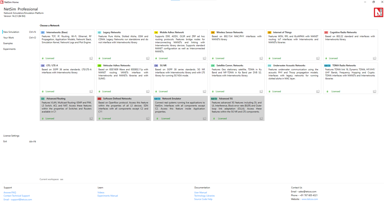
Figure 1‑1: NetSim Home Screen
Network Design Window: A user would enter the design window upon selecting a network type in the home screen. The NetSim design window GUI see Figure 1‑2. It enables users to model a network comprising of network devices like switches, routers, nodes, etc., connect them through links, and model application traffic to flow through the network. The network devices shown in the palette are specific to the network technologies chosen by the user.

Figure 1‑2: Network Design Window
Description:
File - In order to save the network scenario before or after running the simulation into the current workspace,
Click on File 🡪 Save to save the simulation inside the current workspace. Users can specify their own Experiment Name and Description (Optional).
Click on File 🡪 Save As to save an already saved simulation in a different name after performing required modifications to it.
Click on Close, to close the design window or GUI. It will take you to the home screen of NetSim.
Help - Help option allows the users to access all the help features.
Video Tutorials – Assists the users by directing them to our dedicated YouTube Channel “TETCOS”, where we have lots of video presentations ranging from short to long, covering different versions of NetSim up to the latest release.
Answers/FAQ – Assists the user by directing them to our “NetSim Support Portal”, where one can find a well-structured “Knowledge Base”, consisting of answers or solutions to all the commonest queries which a new user can go through.
Raise a Support Ticket – Assists the user by directing them to our “NetSim Support Portal”, where one can “Submit a ticket” or in other words raise his/her query, which reaches our dedicated Helpdesk and due support will be provided to the user.
User Manual – Assists the user with the usability of the entire tool and its features. It highly facilitates a new user with lots of key information about NetSim.
Source Code Help – Assists the user with a structured documentation for “NetSim Source Code Help”, which helps the users who are doing their R&D using NetSim with a structured code documentation consisting of more than 5000 pages with very much ease of navigation from one part of the document to another.
Open-Source Code – Assists the user to open the entire source codes of NetSim protocol libraries in Visual Studio, where one can start initiating the debugging process or performing modifications to existing code or adding new lines of code. Visual Studio Community Edition is a highly recommended IDE to our users who are using the R&D Version of NetSim.
Experiments – Assists the user with separate links provided for 30+ different experiments covering almost all the network technologies present in NetSim.
Technology Libraries – Assists the user by directing them to a folder comprising of individual technology library files comprising all the components present in NetSim.
Below the menu options, the entire region constitutes the Ribbon/Toolbar using which the following actions can be performed:
Click and drop network devices and right click to edit properties.
Click on Wired/Wireless links to connect the devices to one another. It automatically detects whether to use a Wired/Wireless link based on the devices we are trying to connect.
Click on any Application from Set Traffic tab to configure different types of applications and generate traffic.
Click on Plots, Packet Trace, and Event Trace from Configure reports tab to generate metrics to further analyze the network performance.
Click on Run to perform the simulation and specify the simulation time in seconds.
The Show/hide tab is mainly used to display various parameters like Device Name, IP, etc., to provide a better understanding especially during the designing of the scenario.
Results Window: Upon completion of simulation, Network statistics or network performance metrics reported in the form of graphs and tables. The report includes metrics like throughput, simulation time, packets generated, packets dropped, collision counts etc. see Figure 1‑3 and Figure 1‑4.
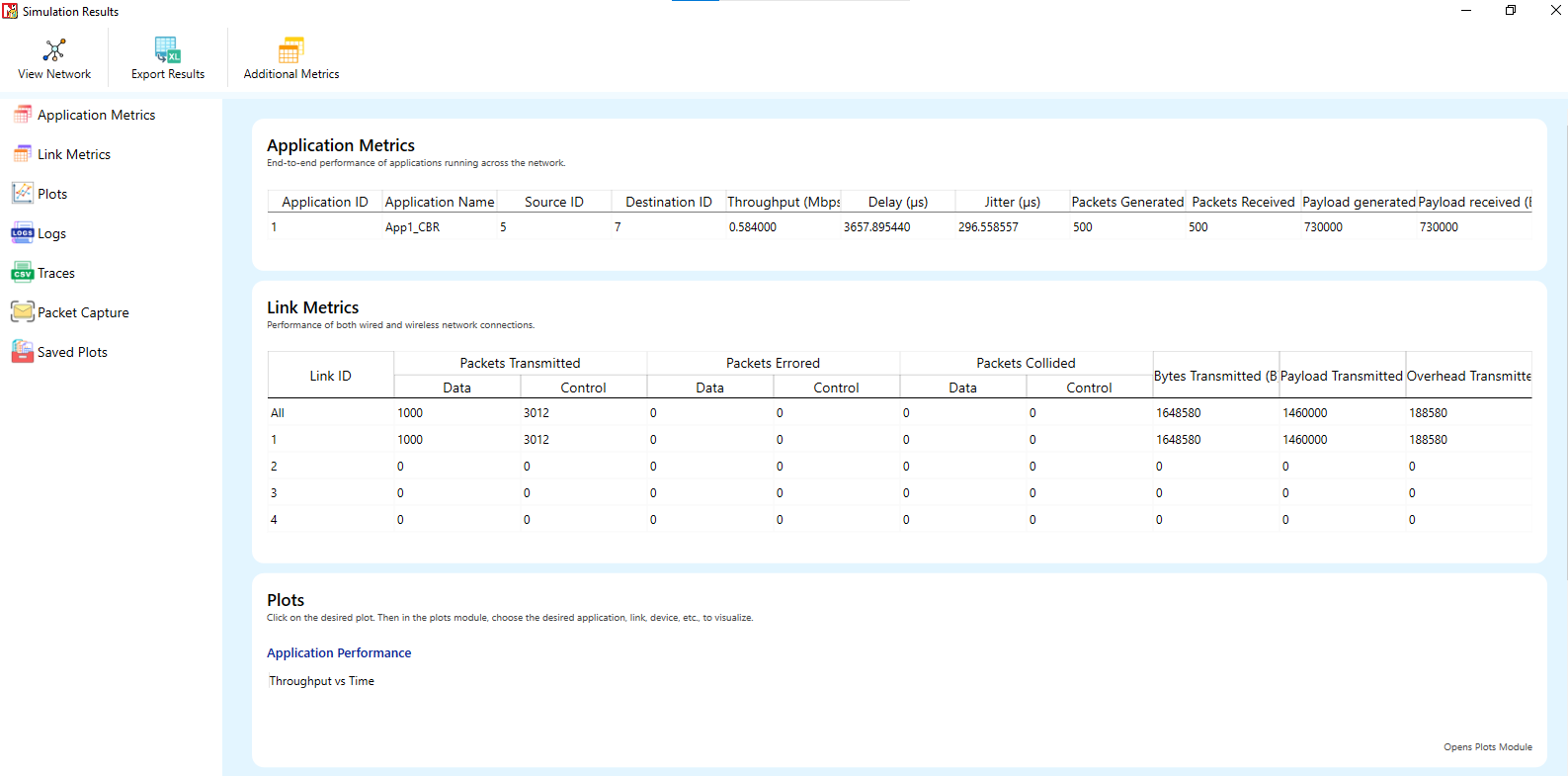
Figure 1‑3: Results Window

Figure 1‑4: Application Throughput Plot
Description:
In the Simulation Results, clicking on a particular metrics will highlight the respective metrics window in the Centre.
Clicking on links in a particular metric link like Plots, Logs, Traces will open the respective files in a separate window.
Click on Packet trace / Event trace to open the csv file which will provide in depth analysis on each Packets / Events.
Users can click on Additional metrics on the top ribbon to view the additional metrics table.
How does a user create and save an experiment in workspace?
To create an experiment, select New simulation-> <Any Network> in the NetSim home screen Figure 1‑5.

Figure 1‑5: NetSim Home Screen
Create a network and save the experiment by clicking on File->Save button on the top left.
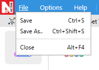
Figure 1‑6: Save the network using file option
A save popup window appears which contains experiment name, workspace path and description see Figure 1‑7.

Figure 1‑7: NetSim Save Window
Specify the Experiment name and description (optional) and then click on save. The workspace path is non-editable. Hence all the experiments will be saved in the default workspace path. After specifying the experiment name click on save.
In our example we saved with the name MANET and this experiment can be found in the default workspace path see below Figure 1‑8.

Figure 1‑8: NetSim Default Workspace Path
Users can also see the saved experiments in “Your work” menu shown below Figure 1‑9.
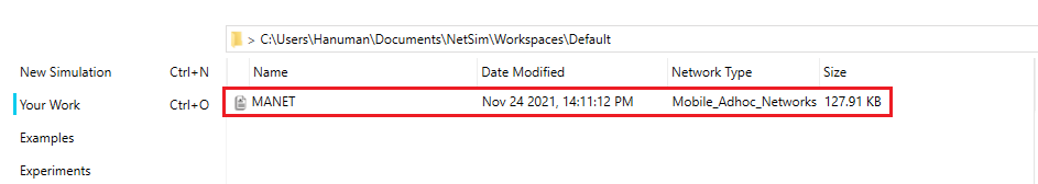
Figure 1‑9: Your Work Menu
“Save As” option is also available to save the current experiment with a different name.
Typical sequence of steps to perform the experiments provided in this manual
The typical steps involved in doing experiments in NetSim are:
Network Set up: Drag and drop devices and connect them using wired or wireless links.
Configure Properties: Configure device, protocol, or link properties by right clicking on the device or link and modifying parameters in the properties window.
Model Traffic: Click on the Application icon present in the Set Traffic tab and set traffic flows.
Enable Trace/Plots (optional): To enable Packet Trace, Event Trace and Plots click on Configure Reports tab and select the respective icons to enable. Packet trace logs packet flow, event trace logs each event (NetSim is a discrete event simulator) and the Plots button enables charting of various throughputs over time.
Save/Save As/Open/Edit: Click on File 🡪 Save / File 🡪 Save As to save the experiments in the current workspace. Saved experiments can then opened from NetSim home screen to run the simulation or to modify the parameters and again run the simulation.
NOTE: Example Configuration files for all experiments would available where NetSim has been installed. This directory is (<NetSim Install Directory>\Docs\Sample Configuration\NetSim Experiment Manual)
Understand the working of basic networking commands - Ping, Route Add/Delete/Print, ACL (Level 1)
Theory
NetSim allows users to interact with the simulation at runtime via a socket or through a file. User Interactions make simulation more realistic by allowing command execution to view/modify certain device parameters during runtime.
Ping Command
The ping command is one of the most often used networking utilities for troubleshooting network problems.
You can use the ping command to test the availability of a networking device (usually a computer) on a network.
When you ping a device, you send that device a short message, which it then sends back (the echo)
If you receive a reply then the device is in the Network, if you do not, then the device is faulty, disconnected, switched off, or incorrectly configured.
Route Commands
You can use the route commands to view, add and delete routes in IP routing tables.
route print: In order to view the entire contents of the IP routing table.
route delete: In order to delete all routes in the IP routing table.
route add: In order to add a static TCP/IP route to the IP routing table.
ACL Configuration
Routers provide basic traffic filtering capabilities, such as blocking the Internet traffic with access control lists (ACLs). An ACL is a sequential list of Permit or Deny statements that apply to addresses or upper-layer protocols. These lists tell the router what types of packets to: PERMIT or DENY. When using an access-list to filter traffic, a PERMIT statement is used to “allow” traffic, while a DENY statement is used to “block” traffic.
Network setup
Open NetSim and click on Experiments> Advanced Routing> Basic networking commands Ping Route Add/Delete/Print and ACL then click on the tile in the middle panel to load the example as shown in below Figure 1‑10.

Figure 1‑10: List of scenarios for the example of Basic networking commands Ping Route Add/Delete/Print and ACL
NetSim UI displays the configuration file corresponding to this experiment as shown below Figure 1‑11.

Figure 1‑11: Network set up for studying the Basic networking commands: Ping, Route Add/Delete/Print, and ACL
Procedure
The following set of procedures were done to generate this sample:
Step 1: A network scenario is designed in NetSim GUI comprising of 2 Wired Nodes and 3 Routers in the “Internetworks” Network Library.
Step 2: Click on Wired Node 1 and then open right-side property panel .In the Network Layer properties of Wired Node 1, “ICMP Status” is set as TRUE.
Similarly, ICMP Status is set as TRUE for all the devices as shown Figure 1‑12.

Figure 1‑12: Network Layer properties of Wired Node 1
Step 3: Click on Wired Node 1 and then open right-side property panel. In the General properties of Wired Node 1, Wireshark Capture is set as Online .
Step 4: Configure an application between any two nodes by selecting a CBR application from Wired Node 1 i.e., Source to Wired Node 2 i.e., Destination from Set Traffic tab in the ribbon. Click on the application, expand the right-side property panel and set Transport Protocol to UDP and Set Packet Size: 1460 Bytes, Inter Arrival Time remaining 233.6µs
Additionally, the “Start Time(s)” parameter is set to 30, while configuring the application. This time is usually set to be greater than the time taken for OSPF Convergence (i.e., Exchange of OSPF information between all the routers), and it increases as the size of the network increases.
Step 5: Packet Trace is enabled in NetSim GUI. At the end of the simulation, a very large .csv file containing the packet information is available for the users to perform packet level analysis.
Step 6: Before simulating the scenario, right click on Router 3 or any other Router and select “NetSim Console” option as shown
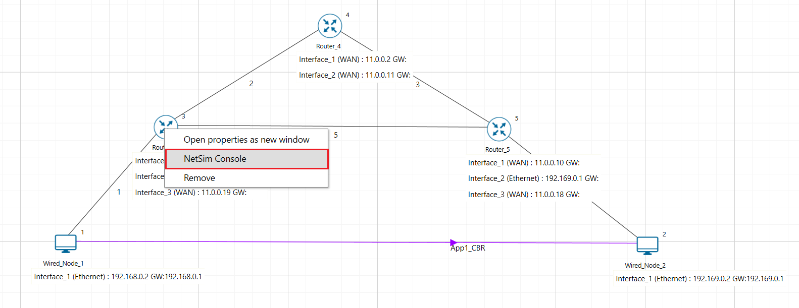
Figure 1‑13: Select NetSim console
Now client (NetSimCLI.exe) will start running and it will try to establish a connection with NetSimCore.exe as shown in Figure 1‑14.

Figure 1‑14: Connection established.
Step 7: Click on options and select Run Time Interactions as shown below

Figure 1‑15: Runtime Interaction window
In the Run time Interaction tab, Interactive simulation option is set to True and click on OK.

Figure 1‑16: Runtime Interaction Simulation window
Click on Run simulation window and simulate it to 300 sec.

Figure 1‑17: Run Simulation Window
NOTE: It is recommended to specify a longer simulation time to ensure that there is sufficient time for the user to execute the various commands and see the effect of that before the Simulation ends.
(NetSimCore.exe) will start running and will display a message “waiting for first client to connect” as shown below.

Figure 1‑18: Waiting for first client to connect.
After this the command line interface can be used to execute all the supported commands.

Figure 1‑19: Connection establishment.
Network Commands
Ping Command
You can use the ping command with an IP address or Device name.
ICMP Status should be set as True in all nodes for ping to work.
Ping <IP address> e.g. ping 192.169.0.2
Ping <Node Name> e.g. ping Wired_Node_2

Figure 1‑20: Pinging Wired Node 2
Route Commands
To view the entire contents of the IP routing table, use following command route print
route print 
Figure 1‑21: IP routing table
You’ll see the routing table entries with network destinations and the gateways to which packets are forwarded when they are headed to that destination. Unless you’ve already added static routes to the table, everything you see here is dynamically generated.
To delete a route in the IP routing table you’ll type a command using the following syntax
route delete destination network So, to delete the route with destination network 11.0.0.18, all we’d have to do is type this command
route delete 11.0.0.18 To check whether route has been deleted or not check again using route print command.
To add a static route to the table, you’ll type a command using the following syntax.
route ADD destination_network MASK subnet_mask gateway_ip metric_cost interface So, for example, if you wanted to add a route specifying that all traffic bound for the 11.0.0.18 subnet went to a gateway at 11.0.0.19
route ADD 192.169.0.2 MASK 255.255.255.255 11.0.0.2 METRIC 1 IF 2 If you were to use the route print command to look at the table now, you’d see your new static route.

Figure 1‑22: Route delete/ Route add
NOTE: Entry added in IP table by routing protocol continuously gets updated. If a user tries to remove a route via route delete command, there is always a chance that routing protocol will re-enter this entry again. Users can use ACL / Static route to override the routing protocol entry if required.
ACL Configuration
Commands to configure ACL
To view ACL syntax: acl print
Before using ACL, we must first verify whether ACL option enabled. A common way to enable ACL is to use command: ACL Enable
Enter configuration mode of ACL: aclconfig
To view ACL Table: Print
To exit from ACL configuration: exit
To disable ACL: ACL Disable (use this command after exit from ACL Configuration)
To view ACL usage syntax use: acl print
[PERMIT, DENY] [INBOUND, OUTBOUND, BOTH] PROTO SRC DEST SPORT DPORT IFID Step to Configure ACL
To create a new rule in the ACL, use command as shown below to block UDP packet in Interface 2 and Interface 3 of Router 3.
Application properties 🡪 Transport Protocol 🡪 UDP as shown Figure 1‑23

Figure 1‑23: Application properties window
Use the command as follows Figure 1‑24.
NetSim>acl enable
ACL is enable
NetSim>aclconfig
ROUTER_3/ACLCONFIG>acl print
Usage: [PERMIT, DENY] [INBOUND, OUTBOUND, BOTH] PROTO SRC DEST SPORT DPORT IFID
ROUTER_3/ACLCONFIG>DENY BOTH UDP ANY ANY 0 0 2
OK!
ROUTER_3/ACLCONFIG>DENY BOTH UDP ANY ANY 0 0 3
OK!
ROUTER_3/ACLCONFIG>print
DENY BOTH UDP ANY/0 ANY/0 0 0 2
DENY BOTH UDP ANY/0 ANY/0 0 0 3
ROUTER_3/ACLCONFIG>exit
NetSim>acl disable
ACL is disable
NetSim>

Figure 1‑24: ACL Configuration command
Ping Command Results
Go to the Results Dashboard and click on “Open Packet Trace” option present in the Left-Hand-Side of the window and do the following:
Filter Control Packet Type/App Name to ICMP EchoRequest and ICMP EchoReply as shown Figure 1‑25.
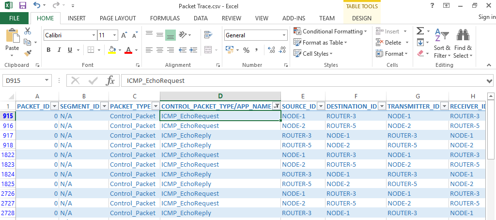
Figure 1‑25: Packet trace - ICMP control packets
In wireshark, apply filter as ICMP. we can see the ping request and reply packets in wireshark as shown Figure 1‑26.

Figure 1‑26: ICMP control packets in wireshark
ACL Results
The impact of ACL rule applied over the simulation traffic can be observed in the IP Metrics Table in the simulation results window. In Router 3, the number of packets blocked by firewall has been shown below Figure 1‑27.

Figure 1‑27: IP Metrics Table from result window
NOTE: Number of packets blocked may vary depending on the time at which ACL is configured.
Exercises
Construct the network scenario shown in the figure below comprising of 5 routers (3 routers in upper path and 2 routers in the lower path) and 2 end nodes. Enable the ICMP protocol in all devices and use the route commands - "route delete" and "route add" - to alter the path for data transfer. The data flow path should be Node1 > R3 > R5 > R6 > R7 > Node2. Enable packet trace and confirm that data indeed flows along this path post simulation.

Figure 1‑28: Network scenario for reference.
Configure the scenario as shown and apply the ACL command as follows.
Apply DENY action for R1 interface 1 and 2.
Apply Permit action for R1 interface 3.
Analyze the firewall blocks in the IP metrics table and explain the throughput results.
Note that ACL commands will only take effect once the commands are entered in the console window.

Figure 1‑29: Network scenario for ACL exercise.
Understand the events involved in NetSim DES (Discrete Event Simulator) in simulating flow of one packet from a Wired node to a Wireless node (Level 2)
Theory
NetSim’s Network Stack forms the core of NetSim, and its architectural aspects are diagrammatically explained below. Network Stack accepts inputs from the end-user in the form of Configuration file and the data flows as packets from one layer to another layer in the Network Stack. All packets, when transferred between devices move up and down the stack, and all events in NetSim fall under one of these ten categories of events, namely, Physical In, Data Link In, Network In, Transport In, Application In, Application Out, Transport Out, Network Out, Data link Out and Physical Out. The IN events occur when the packets are entering a device while the OUT events occur while the packet is leaving a device.
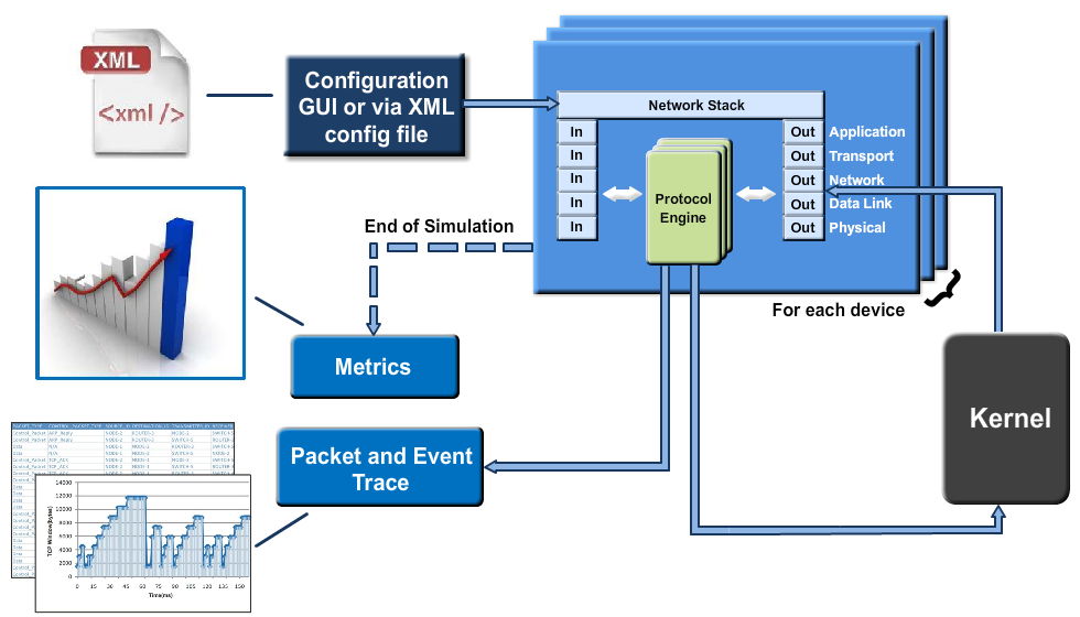
Figure 1‑30: Flow of one packet from a Wired node to a Wireless node
Every device in NetSim has an instance of the Network Stack shown above. Switches & Access points have a 2-layer stack, while routers have a 3-layer stack. End-nodes have a 5-layer stack.
The protocol engines are called based on the layer at which the protocols operate. For example, TCP is called during execution of Transport In or Transport Out events, while 802.11b WLAN is called during execution of MAC IN, MAC OUT, PHY IN and PHY OUT events.
When these protocols are in operation, they in turn generate events for NetSim's discrete event engine to process. These are known as sub events. All sub events fall into one of the above 10 types of events.
Each event gets added in the simulation kernel by the protocol operating at the particular layer of the Network stack. The required sub events are passed into the simulation kernel. These sub events are then fetched by the Network stack in order to execute the functionality of each protocol. At the end of simulation, Network stack writes trace files and the metrics files that assist the user in analyzing the performance metrics and statistical analysis.
Event Trace
The event trace records every single event along with associated information such as time stamp, event Id, event type etc. in a text file or .csv file which can be stored at a user defined location.
Network Setup
Open NetSim and click on Experiments> Internetworks> Network Performance> Advanced Simulation events in NetSim for transmitting one packet then click on the tile in the middle panel to load the example as shown in below Figure 1‑31.

Figure 1‑31: List of scenarios for the example of Advanced Simulation events in NetSim for transmitting one packet.
NetSim UI displays the configuration file corresponding to this experiment as shown below Figure 1‑32.

Figure 1‑32: Network set up for studying the advanced simulation events in NetSim for transmitting one packet.
Procedure
The following set of procedures were done to generate this sample:
Step 1: A network scenario is designed in NetSim GUI comprising of 1 wired node, 1 wireless node, 1 router, and 1 Access point in the “Internetworks” Network library.
Step 2: The device positions are configured according to Table 1‑1 .To set the device positions, click on the device, expand the property panel on the right and change the X and Y co-ordinates in position layer.
Device positions Access Point 2 Wired Node 4 Wireless Node 1 Router 3 X / Lon 150 250 100 200 Y / Lat 50 100 100 50 Table 1‑1: Devices positions
Step 3: Click on link and expand the link property panel on right and set the Channel characteristics to No pathloss.
Step 4: A CBR Application is generated from wired node 4 i.e., source to wireless node 1 i.e., by clicking on set traffic tab from the ribbon on top. The transport protocol is set to UDP by clicking on application and expanding property panel on right.
Step 5: Event Trace is enabled by clicking on configure reports tab from the ribbon on top.
Step 6: Run the simulation for 10 secs. At the end of the simulation, a very large .csv file containing all the UDP IN and OUT EVENTS is available for the users.
NOTE: Event trace is available only in NetSim Standard and Pro versions.
Output
Post simulation, open the event trace from the simulation results window. An Event trace file opens in excel as shown below:

Figure 1‑33: Event trace
We start from the APPLICATION OUT event of the first packet, which happens in the Wired Node and end with the MAC IN event of the WLAN ACK packet which reaches the Wired Node. Events in the event trace are logged with respect to the time of occurrence due to which, event id may not be in order.
Events Involved
Events are listed in the following format:
[EVENT_TYPE, EVENT_TIME, PROTOCOL, EVENT_NO, SUBEVENT_TYPE]
[APP_OUT, 20000, APP, 6, -]
[TRNS_OUT, 20000, UDP, 7, -]
[NW_OUT, 20000, IPV4, 9, -]
[MAC_OUT, 20000, ETH, 10, -]
[MAC_OUT, 20000, ETH, 11, CS]
[MAC_OUT, 20000.96, ETH, 12, IFG]
[PHY_OUT, 20000.96, ETH, 13, -]
[PHY_OUT, 20122.08, ETH, 14, PHY_SENSE]
[PHY_IN, 20127.08, ETH, 15, -]
[MAC_IN, 20127.08, ETH, 16, -]
[NW_IN, 20127.08, IPV4, 17, -]
[NW_OUT, 20127.08, IPV4, 18, -]
[MAC_OUT, 20127.08, ETH, 19, -]
[MAC_OUT, 20127.08, ETH, 20, CS]
[MAC_OUT, 20128.04, ETH, 21, IFG]
[PHY_OUT, 20128.04, ETH, 22, -]
[PHY_OUT, 20249.16, ETH, 23, PHY_SENSE]
[PHY_IN, 20254.16, ETH, 24, -]
[MAC_IN, 20254.16, ETH, 25, -]
[MAC_OUT, 20254.16, WLAN, 26, -]
[MAC_OUT, 20254.16, WLAN, 27, DIFS_END]
[MAC_OUT, 20304.16, WLAN, 28, BACKOFF]
[MAC_OUT, 20324.16, WLAN, 29, BACKOFF]
[MAC_OUT, 20344.16, WLAN, 30, BACKOFF]
[MAC_OUT, 20364.16, WLAN, 31, BACKOFF]
[PHY_OUT, 20364.16, WLAN, 32, -]
[TIMER_EVENT, 21668.16, WLAN, 35, UPDATE_DEVICE_STATUS]
[PHY_IN, 21668.4, WLAN, 33, -]
[MAC_IN, 21668.4, WLAN, 36, RECEIVE_MPDU]
[NW_IN, 21668.4, IPV4, 37, -]
[MAC_OUT, 21668.4, WLAN, 38, SEND_ACK]
[TRNS_IN, 21668.4, UDP, 39, -]
[APP_IN, 21668.4, APP, 41, -]
[PHY_OUT, 21678.4, WLAN, 40, -]
[TIMER_EVENT, 21982.4, WLAN, 43, UPDATE_DEVICE]
[PHY_IN, 21982.63, WLAN, 42, -]
[MAC_IN, 21982.63, WLAN, 44, RECEIVE_ACK]
[TIMER_EVENT, 21985, WLAN, 34, ACK_TIMEOUT]
Event Flow Diagram for one packet from Wired Node to Wireless Node

Figure 1‑34: Event Flow Diagram for one packet from Wired Node to Wireless Node
For Example:
MAC OUT in the Access Point involves sub events like CS, IEEE802.11 EVENT DIFS END and IEEE802.11 EVENT BACKOFF. As you can see in the trace file shown below, CS happens at event time 20252.24. Adding DIFS time of 50µs to this will give IEEE802.11 EVENT DIFS END sub event at 20302.24. Further it is followed by three backoffs each of 20 µs, at event time 20322.24, 20342.24, 020362.24 respectively.

Figure 1‑35: Sub events like CS, IEEE802.11 event DIFS END and IEEE802.11 event BACKOFF event times
In this manner the event trace can be used to understand the flow of events in NetSim Discrete Event Simulator.
Discussion
In NetSim each event occurs at a particular instant in time and marks a change of state in the system. Between consecutive events, no change in the system is assumed to occur. Thus the simulation can directly jump in time from one event to the next.
This contrasts with continuous simulation in which the simulation continuously tracks the system dynamics over time. Because discrete-event simulations do not have to simulate every time slice, they can typically run much faster than the corresponding continuous simulation.
Understanding NetSim’s Event trace and its flow is helpful for source code customization and debugging. The event IDs provided in the event trace can be used to go to a specific event while debugging. This capability is valuable when verifying the correctness of changes made to the source code.
Plot the characteristic curve of throughput versus offered traffic for a Pure and Slotted Aloha system (Level 2)
Theory
ALOHA provides a wireless data network. It is a multiple access protocol (this protocol is for allocating a multiple access channel). There are two main versions of ALOHA: pure and slotted. They differ with respect to whether time is divided up into discrete slots into which all frames must fit.
Pure Aloha
In Pure Aloha, users transmit whenever they have data to be sent. There will be collisions and the colliding frames will then be retransmitted. In NetSim’s Aloha library, the sender waits a random amount of time per the exponential back-off algorithm and sends it again. The frame is discarded when the number of collisions a packet experiences crosses the “Retry Limit” - a user settable parameter in the GUI.
Let ‘‘frame time’’ denotes the amount of time needed to transmit the standard, fixed-length frame. In this experiment point, we assume that the new frames generated by the stations are modeled by a Poisson distribution with a mean of N frames per frame time. If N > 1, the nodes are generating frames at a higher rate than the channel can handle, and nearly every frame will suffer a collision. For reasonable throughput, we would expect 0 < N < 1. In addition to the new frames, the stations also generate retransmissions of frames that previously suffered collisions.
The probability of no other traffic being initiated during the entire vulnerable period is given by\(\ e^{- 2G}\)which leads to \(S = \ G \times e^{- 2G}\) where, S is the throughput and G is the offered load. The units of\(\ S\) and \(G\) is frames per frame time.
G is the mean of the Poisson distribution followed by the transmission attempts per frame time, old and new combined. Old frames mean those frames that have previously suffered collisions.
The maximum throughput occurs at \(G = 0.5\), with \(S = \frac{1}{2e}\), which is about 0.184. In other words, the best we can hope for is a channel utilization of 18%. This result is not very encouraging, but with everyone transmitting at will, we could hardly have expected a 100% success rate.
Slotted Aloha
In slotted Aloha, time is divided up into discrete intervals, each interval corresponding to one frame. In Slotted Aloha, a node is required to wait for the beginning of the next slot in order to send the next packet. The probability of no other traffic being initiated during the entire vulnerable period is given by \(e^{- G}\) which leads to \(S = G \times e^{- G}\). It is easy to compute that Slotted Aloha peaks at G = 1, with a throughput of \(s = \frac{1}{e}\) or about 0.368.
Offered load and throughput calculations1
Using NetSim, the attempts per packet time (G) can be calculated as follows.
\[\ \ G = \ \ \frac{Number\ of\ packets\ transmitted \times PacketTime(s)\ }{SimulationTime\ (s)}\]
where, G is Attempts per packet time. We derive the above formula keeping in mind that (i) NetSim’s output metric, the number of packets transmitted, is nothing but the number of attempts, and (ii) since packets transmitted is computed over the entire simulation time, the number of “packet times” would be \(\frac{SimulationTime(s)}{PacketTransmissionTime(s)}\) , which is in the denominator. Note that in NetSim the output metric Packets transmitted is counted at link (PHY layer) level. Hence MAC layer re-tries are factored into this metric.
The throughput (in Mbps) per packet time can be obtained as follows.
\[\ \ S = \ \ \ \ \frac{Number\ of\ packets\ successful \times PacketTime(s)}{SimulationTime\ (s)}\]
where, S = Throughput per packet time. In case of slotted aloha packet (transmission) time is equal to slot length (time). The packet transmission time is the PHY layer packet size in bits divided by the PHY rate in bits/s. Considering the PHY layer packet size as 1500B, and the PHY rate as 10 Mbps, the packet transmission time (or packet time) would be \(\frac{1500 \times 8}{10 \times 10^{6}} = 1200\ \mu s\).
In the following experiment, we have taken packet size as 1460 B (Data Size) plus 28 B (Overheads) which equals 1488 B. The PHY data rate is 10 Mbps and hence packet time is equal to 1.2 milliseconds.
Network Set Up
Open NetSim and click on Experiments> Legacy Networks> Throughput versus load for Pure and Slotted Aloha> Pure Aloha then click on the tile in the middle panel to load the example as shown in below figure

Figure 1‑36: List of scenarios for the example of Throughput versus load for Pure and Slotted Aloha
NetSim UI displays the configuration file corresponding to this experiment as shown below Figure 1‑37.

Figure 1‑37: Network set up for studying the Pure aloha
Pure Aloha: Input for 0.5 Mbps Generation rate sample
Step 1: Drop 16 nodes (i.e., 15 Nodes are generating traffic.) Node 2 to 16 generates traffic to Node 1. The properties of transmitter nodes which transmits data to Node 1 are given in the below table.
Step 2: Click on the wireless node and expand the property panel on right and set the properties as mentioned in below table.
Wireless Node Properties Interface1 Wireless (PHYSICAL LAYER) Data Rate (Mbps) 10 Interface1 Wireless (DATALINK LAYER) Retry Limit 0 MAC Buffer FALSE Slot Length(µs) 1200 Table 1‑2: Wireless Node Properties
(Note: Slot Length(µs) parameter present only in Slotted Aloha 🡪 Wireless Node Properties 🡪 Interface_1 (Wireless))
Step 3: Click on Adhoc link and expand property panel on right and set channel characteristics to No Path Loss.
Step 4: Configure a custom application from the Set Traffic tab in ribbon on top. The properties are set according to the values given in the below Table 1‑3.
Application 1 Properties Application method Unicast Application type Custom Source Id 2 Destination Id 1 Transport protocol UDP Packet size Distribution Constant Value (Bytes) 1460 Inter Arrival Time Distribution Exponential Packet Inter Arrival Time (µs) 350400 Table 1‑3: For Application 1 Properties
Similarly create 14 more application, i.e., Source Id as 2, 3, 4, 5, 6, 7, 8, 9, 10, 11, 12, 13, 14, 15 and 16 and Destination Id as 1, set Packet Size and Inter Arrival Time as shown in above table.
Step 5: Run the simulation for 10 seconds.
NOTE: Users can refer to Section 3.10 in the user manual for configuring the device properties in all wireless nodes at once using rapid configurator.
Input for 1 Mbps Generation rate sample
Step 1: We increase the network load by increasing the generation rate in both pure and slotted Aloha scenarios.
In the Aloha example, we incrementally increase the total generation rate up to 10 Mbps in steps of 0.5 Mbps, as shown in the table below. Here, the generation rate per node is calculated by dividing the total generation rate by the number of transmitters.
\[Generation\ rate\ (per\ node) = \ \frac{Generation\ rate\ (Total)}{No.of\ Transmitters}\]
Number of nodes generating traffic Generation rate (per node) Mbps Generation rate (In total)
Mbps
Packet size (Bytes) Inter packet arrival time (µs) 15 0.03 0.5 1460 350400 15 0.07 1 1460 175200 15 0.10 1.5 1460 116800 15 0.13 2 1460 87600 15 0.17 2.5 1460 70080 15 0.20 3 1460 58400 15 0.23 3.5 1460 50057 15 0.27 4 1460 43800 15 0.30 4.5 1460 38933 15 0.33 5 1460 35040 15 0.37 5.5 1460 31855 15 0.40 6 1460 29200 15 0.43 6.5 1460 26954 15 0.47 7 1460 25029 15 0.50 7.5 1460 23360 15 0.53 8 1460 21900 15 0.57 8.5 1460 20612 15 0.60 9 1460 19467 15 0.63 9.5 1460 18442 15 0.67 10 1460 17520 Table 1‑4: Table shows the inter packet arrival times for various generation rates in Aloha.
Slotted ALOHA: Input for 0.5 Mbps Generation Rate sample
Step 1: Drop 16 nodes (i.e., 15 Nodes are generating traffic.)
Nodes 2, 3, 4, 5, 6, 7, 8, 9, 10, 11, 12, 13, 14, 15 and 16 transmit data to Node 1 and set properties for nodes and application as mentioned above.
Continue the experiment by increasing the total no of generation rate up to 20 Mbps in the steps of 1 Mbps as shown in the below Table 1‑5.
Number of nodes generating traffic Generation rate (per node) Mbps Generation rate (In total)
Mbps
Packet size (Bytes) IAT (µs) 15 1 0.07 1460 175200 15 2 0.13 1460 87600 15 3 0.20 1460 58400 15 4 0.27 1460 43800 15 5 0.33 1460 35040 15 6 0.40 1460 29200 15 7 0.47 1460 25029 15 8 0.53 1460 21900 15 9 0.60 1460 19467 15 10 0.67 1460 17520 15 11 0.73 1460 15927 15 12 0.80 1460 14600 15 13 0.87 1460 13477 15 14 0.93 1460 12514 15 15 1.00 1460 11680 15 16 1.07 1460 10950 15 17 1.13 1460 10306 15 18 1.20 1460 9733 15 19 1.27 1460 9221 15 20 1.33 1460 8760 Table 1‑5: Table shows the inter packet arrival times for various generation rates in Sl. Aloha
Output
Comparison Table: The values for the total number of packets transmitted and collided are obtained from the NetSim simulation results window after running the simulation. The network statistics are provided in the table below, along with calculation of throughput per packet time (S) and the number of packets transmitted per packet time (G).

Figure 1‑38: Simulation results window showing the No. of packets transmitted and collided.
Pure Aloha:
Total no of nodes generating traffic (in Total) Total number of Packets Transmitted Total number of Packets Collided Successful Packets (Packets Transmitted-Packets Collided) Attempts per packet time(G) Throughput per packet time(S) Throughput per packet time. Theoretical
(S =\(\mathbf{\ }\mathbf{G}\mathbf{*}\mathbf{e}^{\mathbf{- 2}\mathbf{G}}\))
0.5 470 59 411 0.0564 0.0493 0.0504 1 891 162 729 0.1069 0.0875 0.0863 1.5 1299 331 968 0.1558 0.1162 0.1141 2 1759 587 1172 0.2110 0.1406 0.1384 2.5 2159 861 1298 0.2590 0.1558 0.1543 3 2603 1158 1445 0.3123 0.1734 0.1672 3.5 3009 1525 1484 0.3610 0.1781 0.1754 4 3426 1892 1534 0.4111 0.1841 0.1807 4.5 3845 2274 1571 0.4614 0.1885 0.1834 5 4225 2641 1584 0.507 0.1901 0.1839 5.5 4636 3055 1581 0.5563 0.1897 0.1829 6 5010 3469 1541 0.6012 0.4163 0.1806 6.5 5418 3926 1492 0.6501 0.1790 0.1771 7 5800 4346 1454 0.696 0.1745 0.1730 7.5 6154 4698 1456 0.7384 0.1747 0.1686 8 6558 5132 1426 0.7869 0.1711 0.1631 8.5 6938 5548 1390 0.8326 0.1668 0.1575 9 7334 6034 1300 0.8801 0.156 0.1514 9.5 7703 6445 1258 0.9244 0.1510 0.1455 10 8095 6886 1209 0.9715 0.1451 0.1392 Table 1‑6: Total No. of Packets transmitted, Collided, Attempts per packet time and throughput per packet time for Pure Aloha.
Slotted Aloha
Number of nodes generating traffic Total number of Packets Transmitted Total number of Packets Collided Successful Packets (Packets Transmitted-Packets Collided) Attempts per packet time(G) Throughput per packet time(S) Throughput per packet time. Theoretical
(S =\(\mathbf{\ }\mathbf{G}\mathbf{*}\mathbf{e}^{\mathbf{-}\mathbf{G}}\))
1 887 105 782 0.1064 0.0938 0.0957 2 1748 326 1422 0.2097 0.1706 0.1701 3 2568 679 1889 0.3081 0.2267 0.2264 4 3386 1135 2251 0.4063 0.2701 0.2706 5 4155 1581 2574 0.4986 0.3089 0.3028 6 4913 2121 2792 0.5895 0.3350 0.3270 7 5671 2765 2906 0.6805 0.3487 0.3446 8 6377 3356 3021 0.7652 0.3625 0.3560 9 7116 3988 3128 0.8541 0.3754 0.3636 10 7840 4724 3116 0.9408 0.3740 0.3672 11 8495 5343 3152 1.0194 0.3782 0.1327 12 9200 6003 3197 1.104 0.3836 0.1214 13 9847 6683 3164 1.1816 0.3797 0.1112 14 10537 7411 3126 1.2645 0.3750 0.3571 15 11158 8135 3023 1.3390 0.3629 0.3510 16 11737 8791 2946 1.4085 0.3536 0.3444 17 12374 9426 2948 1.4849 0.3536 0.0762 18 13006 10170 2836 1.5608 0.3402 0.3277 19 13575 10875 2700 1.6292 0.324 0.3195 20 14163 11471 2692 1.6996 0.3230 0.0568 Table 1‑7: Total No. of Packets Transmitted, Collided, Throughput per packet time and throughput per packet time for Slotted Aloha
Thus, the following characteristic plot for the Pure Aloha and Slotted Aloha is obtained, which agrees well with the theoretical results.

Figure 1‑39: Throughput vs offered load for Pure Aloha

Figure 1‑40: Throughput vs. Offered load for Slotted Aloha
Exercises
Redo the experiment with PHY data rates of 2 Mbps and 5 Mbps, and then similarly compare the Total number of packets transmitted, Collided, Attempts per packet time, and Throughput per packet time for Pure Aloha and Slotted Aloha. Plot the characteristic curve of the same.
Slot time should be 6000 \(\mu s\) for PHY data rate of 2 Mbps.
Slot time should be 2400 \(\mu s\) for PHY data rate of 5 Mbps.