Network Performance
Data traffic types and network performance measures (Level 1)
Network Performance
Throughput
We begin by understanding the throughput of a flow through a subsystem. A flow is a stream of bits of interest, e.g., all bits flowing through a link in one direction, the bits corresponding to a video stored on a server and playing at a device, etc. A subsystem is any part of the network through which bits can flow, e.g., a link in a network, a subnetwork, a router, an entire network except for the endpoints of a particular flow.

Figure 2‑1: We define the throughput of a flow through a sub system. In the top image, the flow of interest is in blue. In the second figure the sub system is the link and throughput is measured on all flows combined. In the bottom image, again the flow of interest is in blue, while the sub system is a network.
In the context of NetSim, we have:
Application throughput: The subsystem is the entire network, except for the two entities involved in the application, and the flow is the bit stream of that application.
Point-to-point link throughput: The subsystem is the link, and the flow is all the bits flowing through the link in a specified direction.
Let \(A(t)\) be the number of bits of the flow during the interval \(\lbrack 0,t\rbrack\), then the throughput up to\(\ t,\)is equal to \(\ \frac{A(t)}{t}\), and the long-run average throughput is equal to \(\lim_{t \rightarrow \infty}\frac{A(t)}{t}\).
Delay
Delay is reported for an entity, e.g., packets in a stream flowing through a subsystem, a user request (such as a connection setup request), a task such as a file transfer.
Let \(t_{k}\) be the time instant at which delay for the \(k^{th}\)entity starts,
e.g., the time of arrival of a packet at a router, the time of a connection request initiation, the time at which a file transfer is requested.
Let \(u_{k}\)be the time instant at which the delay of the \(k^{th\ }\)entity ends,
e.g., the time at which a packet leaves the router, the time at which a connection request is completed, or the time at which a file transfer is completed.
Then \(d_{k} = u_{k} - t_{k}\)is the delay of the \(k^{th}\)entity among the entities of interest.
e.g., the delay of the \(k^{th}\) packet passing through a router, the delay for the connection set up, or the file transfer delay.
The average delay over last \(K\)entities is equal to
\[\ \frac{1}{K}\sum_{k = (N(K - 1))}^{N}{\ d_{k}}\]
This is called a “moving window” average with a window of \(K\), and will track any changes in the system. As it can be seen, the implementation of the above average requires the storage of the past \(K\)values of \(d_{k}.\)An averaging approach that does not require such storage is the Exponentially Weighted Moving Average (EWMA)
\[\overline{d}(N) = \ \sum_{k = 1}^{N}{(1 - \alpha)^{N - k}\alpha\ d_{k} = \overline{d}(N - 1) + \alpha(d_{N} - \overline{d}}(N - 1))\]
which is roughly like averaging over the past \(1/\alpha\\)values of \(d_{k};\) for example, \(\alpha = 0.001\) gives an averaging window of \(1000.\) The limiting average delay is equal to,
\[\lim_{K \rightarrow \infty}\binom{1}{K}\sum_{k = 1}^{K}{\ d_{k}}\]
This limiting average delay is meaningful if the system is statistically invariant over a long time.


Figure 2‑2: Components of network delay
The following are some examples of the network aspects that determine the delay of an entity.
Packet delay through a router
Processing delay: in moving the packet through the “fabric” to the queue at its exit port.
Queuing delay: at the exit port
Transmission delay: in sending out the packet bits onto the digital transmission link
File transfer delay
Connection set up delay: between the request packet from the user, until the connection is set up and transfer starts.
Data transfer delay is the time taken to transmit all the bytes in the file reliably to the user, so that the user has an exact copy of the file, and the file shows up at the user level in the user’s computer.
Generally, the delay of an entity in a network subsystem will depend on:
the “capacity” of the subsystem (e.g., the bit rate of a link), and
the way the capacity is allotted to the various entities being transmitted over the link.
The delay through a subsystem will include the propagation delay (due to speed of light), router queuing delay, router processing delay, and transmission delay.
Types of Traffic
Elastic Traffic
Elastic traffic is generated by applications that do not have any intrinsic “time dependent” rate requirement and can, thus, be transported at arbitrary transfer rates. For example, the file transfer application only requires that each file be transferred reliably but does not impose a transfer rate requirement. Of course, it is desirable that the file is transferred quickly, but that is not a part of the file transfer application requirement.
The following are the QoS requirements of elastic traffic.
Transfer delay and delay variability can be tolerated. An elastic transfer can be performed over a wide range of transfer rates, and the rate can even vary over the duration of the transfer.
The application cannot tolerate data loss.
This does not mean, however, that the network cannot lose any data. Packets can be lost in the network - owing to uncorrectable transmission errors or buffer overflows - provided that the lost packets are recovered by an automatic retransmission procedure.
Thus, effectively the application would see a lossless transport service. Because elastic sources do not require delay guarantees, the delay involved in recovering lost packets can be tolerated.
Stream Traffic
This source of traffic has an intrinsic “time-dependent” behavior. This pattern must be preserved for faithful reproduction at the receiver. The packet network will introduce delays: a fixed propagation delay and queueing delay that can vary from packet to packet. Applications such as real-time interactive speech or video telephony are examples of stream sources.
The following are typical QoS requirements of stream sources.
Delay (average and variation) must be controlled. Real-time interactive traffic such as that from packet telephony would require tight control of end-to-end delay; for example, for packet telephony the end-to-end delay may need to be controlled to less than 200 ms, with a probability more than 0.99.
There is tolerance for data loss. Because of the high levels of redundancy in speech and images, a certain amount of data loss is imperceptible. As an example, for packet voice 5 to 10% of the packets can be lost without significant degradation of the speech quality.
Featured Examples
Analyzing throughput and file transfer delay for elastic traffic.
Open NetSim and click on Experiments> Internetworks> Network Performance> Analyzing throughput and file transfer delay for elastic traffic and then click on the tile in the middle panel to load the example as shown below.

Figure 2‑3: List of scenarios for the example of Data traffic types and network performance measures
Elastic Traffic is configured as FTP over TCP. We create a network with client, server and 2 routers (R1, R2), and configure an FTP application between client and server.
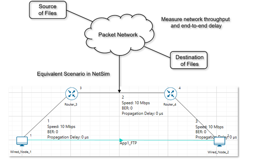
Figure 2‑4: Virtual scenario of FTP application between source and destination created in NetSim.
One file of size 50 MB will be transferred from the server to the client with Application start time = 0, Application end time = 1s. This setting is to ensure that only one file is generated.
We set TCP congestion control algorithm as New Reno with window scaling enabled. Then, in the links, we set BER = 0 and Propagation delay = 0.
Enable packet trace from Configure Reports tab.
Finally, we run the simulation for 100 seconds with (all three) link speeds varying as 10, 20, 50, 75 and 100 Mbps respectively.
| Configuration | Value |
|---|---|
| Network components | Client, Server, R1, R2 |
| Application properties | |
| Traffic type | Elastic traffic configured as FTP over TCP |
| Application start time | 0 |
| Application end time | 1s |
| File size | 50 MB |
| Wired node(Transport layer properties) | |
| Congestion control algorithm | New Reno with window scaling enabled |
| Link settings | |
| Link speed | 10, 20, 50, 75, 100 Mbps |
| Medium property | BER=0, Propagation Delay=0 |
| Simulation time | |
| 100s | |
Table 2‑1: Configuration properties.
Results and discussions
| Link Speed (Mbps) | Application throughput (Mbps) | No. of packets received | Time taken to transfer the entire file in seconds. Simulation output |
\(\mathbf{FileTransferTime}\left( \mathbf{s} \right)\mathbf{\approx}\frac{\left( \mathbf{50 \times 8 \times}\frac{\mathbf{1526}}{\mathbf{1460}} \right)}{\mathbf{LinkSpeed}}\) (Theoretical) |
|---|---|---|---|---|
| 10 | 9.52 | 34247 | 20.98 | 41.80 |
| 20 | 18.98 | 34247 | 10.53 | 20.90 |
| 50 | 47.45 | 34247 | 4.21 | 8.36 |
| 75 | 71.18 | 34247 | 2.80 | 5.57 |
| 100 | 94.92 | 34247 | 2.10 | 4.18 |
Table 2‑2: NetSim results and comparison against theoretical calculations.
Given that the application layer packet size is 1460B packets, a 50 MB file gets fragmented into \(\frac{50 \times 10^{6}}{1460} = 34247\) packets. The PHY layer packet size is equal to \(1460\)B plus \(66\)B of UDP, IP, MAC overheads, which is equal to \(1526\)B. Now, theoretically the
\[FileTransferTime\ (s) = \frac{FileSize(MB) \times 8 \times \left( \frac{PacketSize + OH}{PacketSize} \right)}{LinkSpeed\ (Mbps)}\]
In NetSim, Time taken to transfer the entire file can be computed using the packet trace. It is the time when the last packet was received at the destination less the time at which the file was generated at the source. We see that simulation output agrees well with theory. The slight difference is due to additional time (0.03s) taken for initial connection establishment which is not accounted for in the theoretical calculation.
Figure 2‑5: Throughput and file transfer delay vs. link speed.
Analyzing throughput and delay for stream UDP traffic
Open NetSim and click on Experiments> Internetworks> Network Performance> Analyzing throughput and delay for stream UDP traffic and then click on the tile in the middle panel to load the example as shown below.

Figure 2‑6: List of scenarios for the example of Data traffic types and network performance measures
Stream traffic is configured as streaming video over UDP. We create a scenario with 2 wired nodes (N1, N2), 2 routers (R1, R2). Then, we set the processing delay at routers = 0.
In the links,
Access links (Node-Router): We set the link speed as 100 Mbps, Propagation delay = 0 ms and the BER = 0.
WAN links (Router to Router): We set link speeds as 20 Mbps in cases 1a and 2a, and as 40 Mbps in cases 1b and 2b. Then we set BER = 0, and Propagation delay = 5 ms.
Enable packet trace from Configure Reports tab.
We then simulate two cases as explained below.
Case #1: Configure a video call between N1 and N2
Gen. rate 15 Mbps with Pkt. Size = 1000 B (Const.), and Interarrival time \(\ = \ 533.33\ µs\) (Const.)). Then we set the transport protocol: UDP.
Case #1a: WAN Link (Link # 3) speed = 20 Mbps. Case #1b: WAN link speed = 40 Mbps
Measure throughput and delay
Case #2: Introduce background “load” on the WAN Link, by adding two more nodes (N3, N4) and configuring FTP traffic (over TCP) between them.
We configure a 50 MB file transfer between N3 and N4.
Case #2a: WAN Link (Link # 3) speed = 20 Mbps. Case #2b: WAN link speed = 40 Mbps
Measure throughput and delay

Figure 2‑7: Case 1(a) with WAN link speed of 20 Mbps

Figure 2‑8: Case 1(b) with WAN link speed of 40 Mbps

Figure 2‑9: Case 2(a) with WAN link speed of 20 Mbps

Figure 2‑10: Case 2(b) with WAN link speed of 40 Mbps
Results and observations
| Case # | 1a | 1b | 2a | 2b |
|---|---|---|---|---|
| WAN Link Speed (Mbps) | 20 | 40 | 20 | 40 |
| WAN link Propagation delay (ms) | 5 | 5 | 5 | 5 |
| Total load (Mbps) | 15Mbps video | 15 Mbps video | 15 Mbps video + 50 MB file | 15 Mbps video + 50 MB file |
| Avg. propagation delay (µs). (Three entries, one per link) | 0 + 5000 + 0 |
0 + 5000 + 0 |
0 + 5000 + 0 |
0 + 5000 + 0 |
| Avg. pkt. transmission time (µs) | 84.32 + 411.2 + 84.32 | 84.32 + 205.6 + 84.32 | 84.32 + 411.2 + 84.32 |
84.32 + 205.6 + 84.32 |
| Avg. Queuing Delay (µs) | 0 | 0 | 0+93395.4+0 | 0+1836.82+0 |
| FTP File transfer Time (s) | N/A | N/A | 89.39 | 16.74 |
| Video End-to-end application throughput (Mbps) | 14.99 | 14.99 | 14.99 | 14.99 |
| Video Avg. end-to-end Pkt. Delay (µs) | 5579.84 | 5374.24 | 98975.24 | 7211.07 |
| FTP End-to-end application throughput (Mbps) | N/A | N/A | 4.47 | 23.88 |
Table 2‑3: Results of the 4 different cases.

Figure 2‑11: Throughput and delay values of case 2(b) from results dashboard.
Since traffic is a stream of packets, all delay calculations are based on the average of the metric taken over all packets. In case 2a and 2b, we have a 50 MB File that is transferred from N3 to N4. It uses the same WAN link that video does. We see that,
\[Avg.\ End\ to\ End\ Delay = Avg.queuing\ delay\ + Avg.transmission\ time + Avg.propagation\ delay\]
For FTP we observe that
\[File\ Transfer\ Time(s) \times FTP\ Throughput(Mbps) = File\ size\ (MB) \times 8\]
i.e,
\[89.39 \times 4.47 = 50 \times 8\]
\[399.57 \approx 400\]
where the factor of 8 is for byte to bit conversion.
Throughput Plots

Figure 2‑12: Case 1(a) - WAN (bottleneck) link speed is 20 Mbps.

Figure 2‑13: Case 1(b) - WAN (bottleneck) link speed is 40 Mbps.
We observe that:
In both cases video sees a steady throughput of 15 Mbps
No queuing since the link capacity is 20 Mbps in case 1a and 40 Mbps in case 1b.
From the Table 2‑3 we see that the transmission time is lower in case 1b since it uses a 40 Mbps link.

Figure 2‑14: Case 2(a) - WAN (shared) link capacity is 20 Mbps. Video sees 15 Mbps while FTP gets ≈ 5 Mbps during the file transfer.

Figure 2‑15: Case 2(b) - WAN (shared) link capacity is 40 Mbps. Video sees 15 Mbps while FTP gets ≈ 25 Mbps during the file transfer.
We observe the following:
Case 2(a)
Shared link 20 Mbps with video rate 15 Mbps and file transfer
Video throughput is 15 Mbps and FTP throughput is 5 Mbps during transfer.
Case 2(b)
Shared link 40 Mbps with video rate 15 Mbps and file transfer
Video throughput is 15 Mbps and FTP throughput is 25 Mbps during transfer.
This clearly shows us that the FTP transfer uses TCP which “adapts” to the “remaining” bandwidth.
Analyzing TCP vs. UDP Performance in Error-Prone Network Conditions
Open NetSim and click on Experiments> Internetworks> Network Performance> Analyzing TCP vs. UDP Performance in Error-Prone Network Conditions and then click on the tile in the middle panel to load the example as shown below.
In this example, we observe the impact of link errors on the performance of TCP-based applications compared to UDP-based applications.
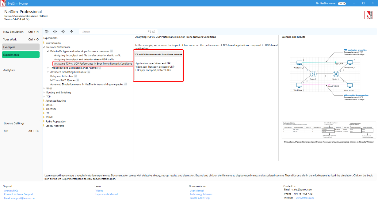
Figure 2‑16: List of scenarios for the example of Data traffic types and network performance measures.
Network Scenario

Figure 2‑17: Network scenario with WAN link speed of 40 Mbps.
Network settings:
Create a Scenario with 4 wired nodes and 2 routers connected as shown above Figure 2‑17.
Set the Wired Link properties, for Link ID 1,2,4,5
Uplink/Downlink speed to 100 Mbps
Uplink/Downlink BER to 0
Propagation delay to 0 µs.
Set the WAN Link properties as below, that Link ID 3 between router 5 and router 6
Uplink/Downlink speed to 40 Mbps
Uplink/Downlink BER to 0.0000005
Propagation delay to 5000 µs.
Create two traffic flows, one running TCP and another running UDP as shown below.
VIDEO application
| Parameter name | Value |
|---|---|
| Application Type | Custom |
| Source Id | 1 |
| Destination Id | 2 |
| Transport protocol | UDP |
| Packet size (B) | 1000 |
| Inter Arrival Time (µs) | 533.3333 |
| Generation rate (Mbps) | 15 |
Table 2‑4: VIDEO Application properties.
File Transfer Application
| Parameter Name | Value |
|---|---|
| Application Type | FTP |
| Source Id | 3 |
| Destination Id | 4 |
| End time (s) | 1 |
| Transport protocol | TCP |
| File size (B) | 50000000 |
| Inter Arrival time (s) | 5 |
| Generation rate (Mbps) | 80 |
Table 2‑5: FTP Application Properties.
Go to Configure Reports Tab > Enable Packet Trace.
Run the Simulation for 150 seconds.
Results and observations
Application Metrics

Figure 2‑18: Throughput, packet generated and packet received show in Application metrics in results window.
UDP achieves a throughput of \(14.96\\)Mbps, while TCP achieves a throughput of \(2.67\) Mbps.
UDP achieves a higher throughput than TCP since UDP doesn’t need to wait for acknowledgements in the reverse direction.
However, in UDP several packets (\(281,251 - 280,057 = 1,194)\)are lost due to error, while TCP all packets are received since TCP retransmits packets errored. The table below shows the number of errored packets that were retransmitted by TCP.

Figure 2‑19: TCP Metrics from Result dashboard > Additional metrics.
Appendix: Obtaining delay metrics in NetSim
The Avg end-to-end packet delay can be got directly from the delay column in the application metrics of NetSim Results dashboard. Queuing delay, transmission time and propagation delay can be calculated from the packet trace which is explained in Section 2.1.4.1.
In the packet trace:
The average of difference between the PHY LAYER ARRIVAL TIME\(\ (µs)\) and the NW LAYER ARRIVAL TIME\(\ (µs)\) will give us the average queuing delay of packets in a link.
\[Avg.Queuing\ delay\ (\mu s) = Avg.\ \left( PHY\ LAYER\ ARRIVAL\ TIME\ (µs) - NW\ LAYER\ ARRIVAL\ TIME\ (µs) \right)\]
The average of difference between the PHY LAYER START TIME \((µs)\) and the PHY LAYER ARRIVAL TIME \((µs)\) will give us the average transmission time of packets in a link.
\[Avg.Transmission\ Time\ (\mu s) = Avg.\left( PHY\ LAYER\ START\ TIME\ (µs) - PHY\ LAYER\ ARRIVAL\ TIME\ (µs) \right)\]
The average of difference between the PHY LAYER END TIME \((µs)\) and the PHY LAYER START TIME \((µs)\) will give us the average propagation delay of packets in a link.
\[Avg.\ Propagation\ delay\ (\mu s) = Avg.\ \left( PHY\ LAYER\ END\ TIME\ (µs) - PHY\ LAYER\ START\ TIME\ (µs) \right)\]
The procedure for calculating \(\mathbf{Avg}\mathbf{.\ }\mathbf{Queuing}\mathbf{\ }\mathbf{delay}\mathbf{\ (}\mathbf{\mu s}\mathbf{)}\)
Consider case 2(b),
To compute average queuing delay, we have to take the avg. queuing delay in each link (2, 3, 5) and take the sum of the delays.
Open Packet Trace file using the Open packet trace option available in the Simulation Results window.
In the Packet Trace, filter the data packets using the column Control Packet Type/App Name to option App1 Video (see Figure 2‑43).

Figure 2‑20: Filter the data packets in Packet Trace by selecting App1 video.
Now, to compute the average queue in Link 3, we will select Transmitter Id as Router-5 and Receiver Id as Router-6. This filters all the successful packets from Router 5 to Router 6.
The columns Network Layer Arrival Time(µS) and Phy Layer Arrival Time(µS) correspond to the arrival time and departure time of the packets in the buffer at Link 3, respectively (see Figure 2‑44).

Figure 2‑21: Packet arrival and departure times in the link buffer
The difference between the Phy Layer Arrival Time(µS) and the Network Layer Arrival Time (µS) will give us the delay of a packet in the link (see Figure 2‑45).
\[Queuing\ Delay = \ Phy\ layer\ arrival\ time(µS) - \ NW\ layer\ arrival\ time(µS)\]
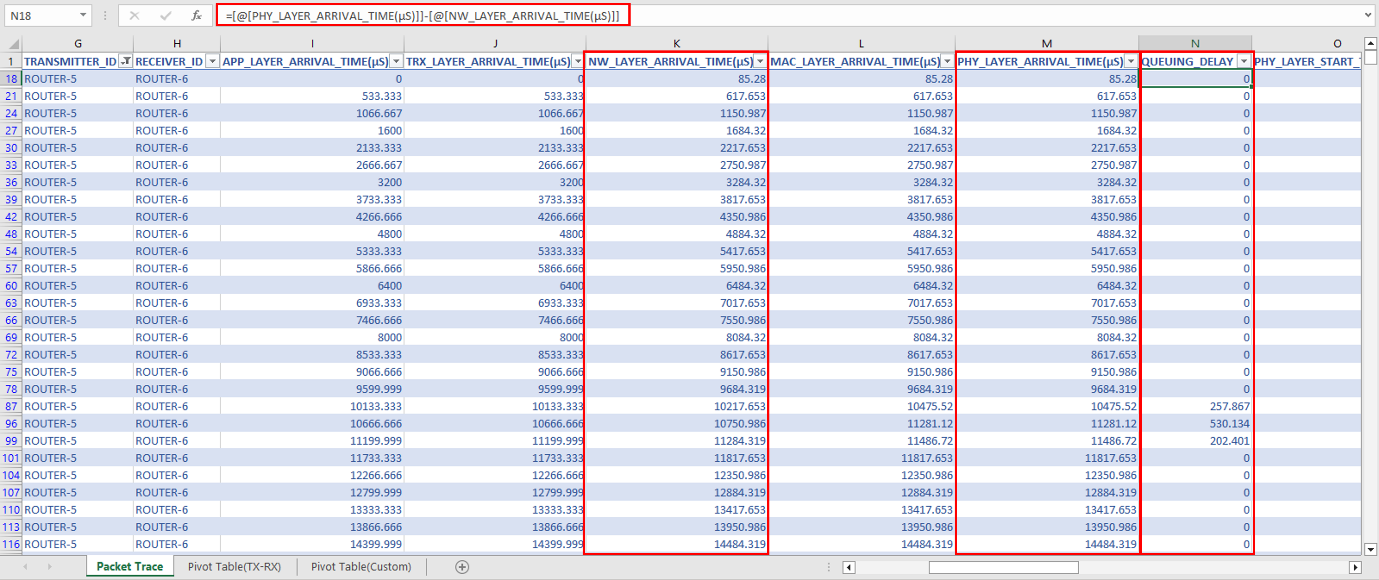
Figure 2‑22: Queuing Delay
Now, calculate the average queuing delay by taking the mean of the queueing delay of all the packets (see Figure 2‑45)

Figure 2‑23: Average queuing delay
The average queuing delay obtained in the packet trace is 1836.82 \(\mu s\) which is same as that as mentioned in Table 2‑3. Similarly, after computing queuing delay for link 2 and link 5 we get avg. queuing delay = 0. Hence the average queuing delay in the network is 1836.82 µs.
Similar steps can be followed to obtain \(Avg.\ Transmission\ Time\ (\mu s)\) and \(Avg.\ Propagation\ Delay\ (\mu s)\).
The procedure for calculating \(\mathbf{File}\mathbf{\ }\mathbf{Transfer}\mathbf{\ }\mathbf{Time}\mathbf{(}\mathbf{s}\mathbf{)}\)
To calculate the File Transfer Time, filter the data packets using the column Control Packet Type/App Name to option App2 FTP
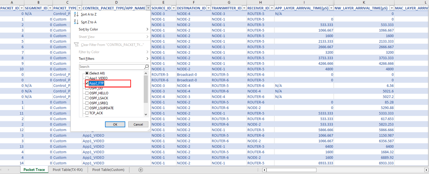
Figure 2‑24: Filter the data packets in Packet Trace by selecting App2_FTP.
Calculate the difference between the last value of Phy layer end time and first value of App layer arrival time.
\[FTP\ file\ transfer\ Time\ (s)\ = \left( Phy\ layer\ end\ time\ (µs) - App\ layer\ arrival\ time\ (µs) \right)\]
\[= 16742892.32\ \mu s - 0\mu s = 16.74s\]

Figure 2‑25: File Transfer Time
Exercises
Redo the experiment by using the following inputs.
Part-A:
Consider the application layer file size of 50 MB and modify the link speed as 120Mbps. Derive the theoretical File transfer time and compare against NetSim result.
For variations, consider different combinations of file sizes, such as 20 MB, 30MB, 40MB, 60MB, 70MB etc., and different link speeds such as 10 Mbps, 50 Mbps, 200 Mbps etc. Derive the theoretical File transfer time for each case and compare against NetSim result.
Part-B:
Redo the experiment mentioned in part-B with customized video traffic generation rate set to 20 Mbps with packet size = 1000B, IAT = 400µs. Derive the theoretical File transfer time for each case and compare against NetSim result obtained using the packet trace.
Redo the experiment mentioned in part-B and generate FTP traffic with 10 MB file size (application settings: File size = 10000000B, IAT = 5s) and a link speed of 50 Mbps. Derive the theoretical File transfer time for each case and compare against NetSim result obtained using the packet trace.
Simulating Link Failure (Level 1)
Objective
To model link failure, understand its impact on network performance
Theory
A link failure can occur due to a) faults in the physical link and b) failure of the connected port. When a link fails, packets cannot be transported. This also means that established routes to destinations may become unavailable. In such cases, the routing protocol must recompute an alternate path around the failure.
In NetSim, only WAN links (connecting two routers) can be failed. Click on a WAN link between two routers and the Link Properties Window is as shown below Figure 2‑26.

Figure 2‑26: Wired Link Properties Window
Link up Time refers to the time(s) at which the link is functional and Link down time refers to the time (s) at which a link fails. Click on up time or down time to understand the configuration options.
NOTE: Link failure can be set only for “WAN Interfaces”.
Network Setup
Open NetSim and click on Experiments> Internetworks> Network Performance> Advanced Simulating Link Failure then click on the tile in the middle panel to load the example as shown in below Figure 2‑27.

Figure 2‑27: List of scenarios for the example of Advanced Simulating Link Failure
Link Failure Single WAN Interface
NetSim UI displays the configuration file corresponding to this experiment as shown below Figure 2‑28.

Figure 2‑28: Network set up for studying the Link Failure Single WAN Interface
Procedure
The following set of procedures were done to generate this sample:
Step 1: In the “Internetworks” library, and a network scenario is designed in NetSim comprising of 2 Wired Nodes and 2 Routers.
Step 2: By default, Link Failure Up time is set to 0,10,20 and Down time is set to 5,15. This means the link is up 0-5s, 10-15s and 20s onwards, and it is down 5-10s and 15-20s. This can set by clicking on WAN link between routers (link 2) and expanding the link property panel on right and changing the link up and link down as shown below.
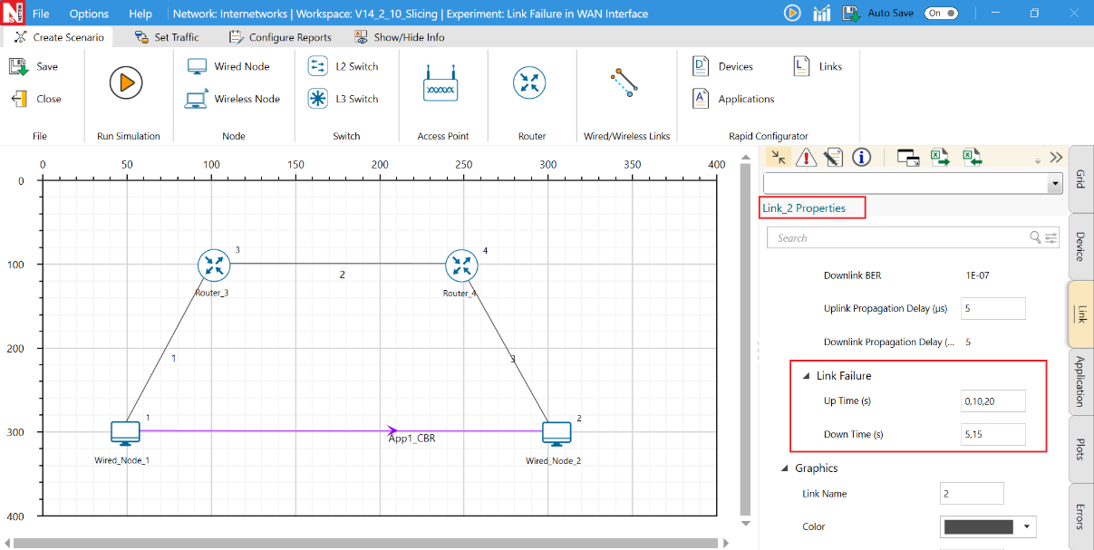
Figure 2‑29: Link failure setting in WAN link
Step 3: Packet trace is enabled from Configure reports tab in the ribbon on the top. At the end of the simulation, a .csv file containing all the packet information is available for performing packet level analysis.
Step 4: Configure a CBR application between wired node 1 to wired node 2 by clicking on set traffic tab in the ribbon on the top. Click on the created application, expand the application property panel on the right, and set the transport layer to UDP while keeping the other properties as default.
Step 5: Enable the Link Throughput vs. Time plot by clicking on Configure reports and plots, then run the simulation for 50 seconds.
Output
Open the Link Throughput plot from the simulation results window, filter the link id to 2 and disable the accelerate plotting and change the average window size to 50ms, we can notice the following.

Figure 2‑30: Link Throughput vs Time plot for Link 2.
The application starts at the 0th second between Router 3 and Router 4 and is initially active from 0 to 5 seconds. A throughput of 0.71 Mbps is observed during the intervals of 0-5 seconds, 10-15 seconds, and from 20 seconds onward.
The link fails in the intervals 5-10s and 15-20s. The throughput drops to 0 Mbps in these intervals.
Similarly, the same can be observed in the packet trace by filtering Control packet type/App name to App1 CBR, Transmitter Id to router 3, and Receiver Id to router 4. By observing the arrival times, you'll notice that no data transmission occurs during the link failure period.

Figure 2‑31: NetSim packet trace showing the link failure period
Link Failure with OSPF
NetSim UI displays the configuration file corresponding to this experiment as shown in Figure 2‑32.

Figure 2‑32: Network set up for studying the Link Failure with OSPF
Procedure
Without link failure: The following set of procedures were done to generate this sample:
Step 1: In the “Internetworks” library, and a network scenario is designed in NetSim comprising of 2 Wired Nodes and 7 Routers.
Step 2: By default, Link Failure Up Time is set to 0 and Down Time is set to 100000 for Link id 3.
Step 3: Packet Trace is enabled from configure reports tab in ribbon on the top. At the end of the simulation, a .csv file containing all the packet information is available for performing packet level analysis.
Step 4: Configure a CBR application between wired node 1 to Wired Node 2 by clicking on set traffic tab in the ribbon on the top. Click on the created application, expand the application property panel on the right, and set the transport layer to TCP.
Additionally, the “Start Time(s)” parameter is set to 30 s. This time is usually set to be greater than the time taken for OSPF convergence (i.e., exchange of OSPF information between all the routers), and it increases as the size of the network increases.
Step 5: Enable the Link Throughput vs. Time plot by clicking on Configure reports and Plots and run the simulation for 80 Seconds.
With link failure: The following changes in settings are done from the previous sample:
Step 1: In Link 3 Properties, Link Failure Up Time is set to 0 and Down Time is set to 50. This means that the link would fail at 50 Seconds.
Step 2: Enable the plots and run the simulation for 80 Seconds.
Output
Open Packet trace and observe the packet flow.
Initially OSPF Control Packets are exchanged between all the routers.
Once after the exchange of control packets, the data packets are sent from the source to the destination.
The packets are routed to the Destination via, N1 > R3 > R4 > R5 > R9 > N2 as shown below Figure 2‑33.
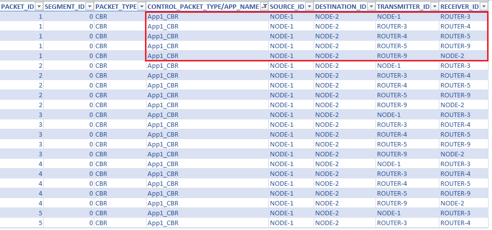
Figure 2‑33: Packet Trace file for without link failure
With link failure
We create a Link Failure in Link 3, between Router 4 and Router 5 at 50s.
Since the packets are not able to reach the destination, the routing protocol recomputes an alternate path to the Destination.
This can be observed in the Packet Trace.
Go to the Results Dashboard and click on Packet Trace under traces and do the following:
Filter Control Packet Type/App Name to APP1 CBR and Transmitter ID to Router 3.
We can notice that packets are changing its route from, N1 > R3 > R4 > R5 > R9 > N2 to N1 > R3 > R6 > R7 > R8 > R9 > N2 at 50 s of simulation time, since the link between R4 and R5 fails at 50 s.
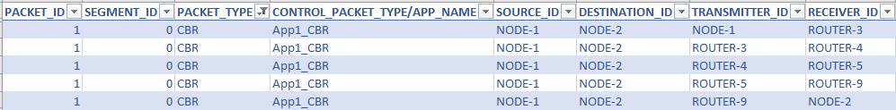
Figure 2‑34: Packet Trace file for link failure before 50 secs

Figure 2‑35: Packet Trace file for link failure after 50 secs
Delay and Little’s Law (Level 2)
Introduction
Delay is another important measure of quality of a network, very relevant for real-time applications. The application processes concern over different types of delay - connection establishment delay, session response delay, end-to-end packet delay, jitter, etc. In this experiment, we will review the most basic and fundamental measure of delay, known as end-to-end packet delay in the network. The end-to-end packet delay denotes the sojourn time of a packet in the network and is computed as follows. Let \(a_{i}\)and \(d_{i}\) denote the time of arrival of packet \(i\) into the network (into the transport layer at the source node) and time of departure of the packet \(i\) from the network (from the transport layer at the destination node), respectively. Then, the sojourn time of the packet i is computed as (\(d_{i} - a_{i}\) ) seconds. A useful measure of delay of a flow is the average end-to-end delay of all the packets in the flow, and is computed as
\[average\ packet\ delay = \frac{1}{N}\sum_{i = 1}^{N}\left( d_{i - \ }a_{i}^{\ } \right)secs\]
where N is the count of packets in the flow.
A packet may encounter delay at different layers (and nodes) in the network. The transport layer at the end hosts may delay packets to control flow rate and congestion in the network. At the network layer (at the end hosts and at the intermediate routers), the packets may be delayed due to queues in the buffers. In every link (along the route), the packets see channel access delay and switching/forwarding delay at the data link layer, and packet transmission delay and propagation delay at the physical layer. In addition, the packets may encounter processing delay (due to hardware restrictions). It is a common practice to group the various components of the delay under the following four categories: queueing delay (caused due to congestion in the network), transmission delay (caused due to channel access and transmission over the channel), propagation delay and processing delay. We will assume zero processing delay and define packet delay as
\[end\ to\ end\ packet\ delay\ = queueing\ delay + transmission\ delay\ + \ propagation\ delay\]
We would like to note that, in many scenarios, the propagation delay and transmission delay are relatively constant in comparison with the queueing delay. This permits us (including applications and algorithms) to use packet delay to estimate congestion (indicated by the queueing delay) in the network.
Little’s Law
The average end-to-end packet delay in the network is related to the average number of packets in the network. Little’s law states that the average number of packets in the network is equal to the average arrival rate of packets into the network multiplied by the average end-to-end delay in the network, i.e.,
\[average\ number\ of\ packets\ in\ the\ network = average\ arrival\ rate\ into\ the\ network \times average\ end\ to\ end\ delay\ in\ the\ network\]
Likewise, the average queueing delay in a buffer is also related to the average number of packets in the queue via Little’s law.
\[average\ number\ of\ packets\ in\ queue = average\ arrival\ rate\ into\ the\ queue \times average\ delay\ in\ the\ queue\]
The following figure illustrates the basic idea behind Little’s law. In Figure 2‑36a, we plot the arrival process \(a(t)\) (thick black line) and the departure process \(d(t)\) (thick red line) of a queue as a function of time. We have also indicated the time of arrivals \((a_{i})\) and time of departures \((d_{i})\) of the four packets in Figure 2‑36a. In Figure 2‑36b, we plot the queue process \(q(t) = a(t) - d(t)\) as a function of time, and in Figure 2‑36c, we plot the waiting time \(\left( d_{i - \ }a_{i}^{\ } \right)\) of the four packets in the network. From the figures, we can note that the area under the queue process is the same as the sum of the waiting time of the four packets. Now, the average number of packets in the queue ( \(\frac{14}{10}\) ) , if we consider a duration of ten seconds for the experiment) is equal to the product of the average arrival rate of packets \(\left( \frac{4}{10} \right)\) and the average delay in the queue \(\left( \frac{14}{4} \right)\).

Figure 2‑36: Illustration of Little’s law in a queue.
In Experiment 3 (Throughput and Bottleneck Server Analysis), we noted that bottleneck server analysis can provide tremendous insights on the flow and network performance. Using M/G/1 analysis of the bottleneck server and Little’s law, we can analyze queueing delay at the bottleneck server and predict end-to-end packet delay as well (assuming constant transmission times and propagation delays).
NetSim Simulation Setup
Open NetSim and click on Experiments> Internetworks> Network Performance> Delay and Littles Law then click on the tile in the middle panel to load the example as shown below in Figure 2‑37.

Figure 2‑37: List of scenarios for the example of Delay and Littles Law
Part-1: A Single Flow Scenario
We will study a simple network setup with a single flow illustrated in Figure 2‑38 to review end to end packet delay in a network as a function of network traffic. An application process at Wired Node 1 seeks to transfer data to an application process at Wired Node 2. We will consider a custom traffic generation process (at the application) that generates data packets of constant length (say, L bits) with IAT inter-arrival times (say, with average inter-arrival time \(v\) seconds). The application traffic generation rate in this setup is \(\frac{L}{v}\) bits per second. We prefer to minimize communication overheads (including delay at the transport layer) and hence, will use UDP for data transfer between the application processes.
In this setup, we will vary the traffic generation rate \(\left( \frac{L}{v} \right)\) by varying the average inter-arrival time \((v)\), and review the average queue at the different links, average queueing delay at the different links and end-to-end packet delay.
Procedure
We will simulate the network setup illustrated in Figure 2‑38 with the configuration parameters listed in detail in Table 2‑6 to study the single flow scenario.
NetSim UI displays the configuration file corresponding to this experiment as shown below:

Figure 2‑38: Network set up for studying a single flow
The following set of procedures were done to generate this sample:
Step 1: Drop two wired nodes and two routers onto the simulation environment. The wired nodes and the routers are connected to wired links as shown in (See Figure 2‑38).
Step 2: Configure an application between any two nodes by selecting a Custom application from the Set Traffic tab. Right click on the Application Flow App1 CBR and select Properties. In the Application configuration window (see Figure 2‑39), select Transport Protocol as UDP. In the PACKET SIZE tab, select Distribution as CONSTANT and Value as 1460 bytes. In the INTER ARRIVAL TIME tab, select Distribution as EXPONENTIAL and Mean as 11680 microseconds.

Figure 2‑39: Application configuration window
Step 3: The properties of the wired nodes are left to the default values.
Step 4: Right-click the link ID (of a wired link) and select Properties to access the link’s properties window (see Figure 2‑40). Set Max Uplink Speed and Max Downlink Speed to 10 Mbps for link 2 (the backbone link connecting the routers) and 1000 Mbps for links 1 and 3 (the access link connecting the Wired_Nodes and the routers).
Set Uplink BER and Downlink BER as 0 for links 1, 2 and 3. Set Uplink Propagation Delay and Downlink Propagation Delay as 0 microseconds for the two-access links 1 and 3 and 10 milliseconds for the backbone link 2.

Figure 2‑40: Link_ID_2 Properties window
Step 5: Right-click Router 3 icon and select Properties to access the link’s properties window (see Figure 2‑41). In the INTERFACE 2 (WAN) tab, select the NETWORK LAYER properties, set Buffer size (MB) to 8.

Figure 2‑41: Router Properties window
Step 6: Enable Packet Trace check box. Packet Trace can be used for packet level analysis.
Step 7: Click on Run icon to access the Run Simulation window (see Figure 2‑42) and set the Simulation Time to 100 seconds and click on Run.

Figure 2‑42: Run Simulation window
Step 8: Now, repeat the simulation with different average inter-arrival times (such as 5840 µs, 3893 µs, 2920 µs, 2336 µs and so on). We vary the input flow rate by varying the average inter-arrival time. This should permit us to identify the bottleneck link and the maximum achievable throughput.
The detailed list of network configuration parameters is presented in (See Table 2‑6).
| Parameter | Value |
|---|---|
| LINK PARAMETERS | |
| Wired Link Speed (access link) | 1000 Mbps |
| Wired Link Speed (backbone link) | 10 Mbps |
| Wired Link BER | 0 |
| Wired Link Propagation Delay (access link) | 0 |
| Wired Link Propagation Delay (backbone link) | 10 milliseconds |
| APPLICATION PARAMETERS | |
| Application | Custom |
| Source ID | 1 |
| Destination ID | 2 |
| Transport Protocol | UDP |
| Packet Size – Value | 1460 bytes |
| Packet Size – Distribution | Constant |
| Inter Arrival Time – Mean | AIAT (µs) Table 2‑26 |
| Inter Arrival Time – Distribution | Exponential |
| ROUTER PARAMETERS | |
| Buffer Size -Interface(WAN) | 8 |
| MISCELLANEOUS | |
| Simulation Time | 100 Sec |
| Packet Trace | Enabled |
Table 2‑6: Detailed Network Parameters
Performance Measure
In Table 2‑7 and Table 2‑9, we report the flow average inter-arrival time v and the corresponding application traffic generation rate, input flow rate (at the physical layer), average queue and delay of packets in the network and in the buffers, and packet loss rate.
Given the average inter-arrival time \(v\) and the application payload size L bits (here, 1460×8 = 11680 bits), we have,
\[Traffic\ generation\ rate = \frac{L}{v} = \frac{11680}{v}bps\]
\[PHY\ rate = \frac{11680 + 54 \times 8}{v} = \frac{12112}{v}bps\]
where the packet overheads of 54 bytes is computed as \(54 = 8(UDP\ header) + 20(IP\ header) + 26(MAC + PHY\ header)\ bytes\).
Let \(Q_{l}(u)\) as denote the instantaneous queue at link \(l\) at time \(u\) . Then, the average queue at link \(l\) is computed as
\[average\ queue\ at\ link\ l = \frac{1}{T}\int_{0}^{T}{Q_{l\ \ }(u)}\ \ du\ bits\]
where, T is the simulation time. And, let \(N(u)\) denote the instantaneous number of packets in the network at time \(u\). Then, the average number of packets in the network is computed as
\[average\ number\ of\ packet\ in\ the\ network\ = \frac{1}{T}\int_{0}^{T}{N(u)}\ \ du\ bits\]
Let \(a_{i,l}\) and \(d_{i,l}\) denote the time of arrival of a packet \(i\) into the link \(l\) (the corresponding router) and the time of departure of the packet \(i\) from the link \(l\) (the corresponding router), respectively. Then, the average queueing delay at the link \(l\) (the corresponding router) is computed as
\[average\ queueing\ delay\ at\ link\ l = \frac{1}{N}\sum_{i = 1}^{N}\left( d_{i,l - \ }a_{i,l}^{\ } \right)\]
where N is the count of packets in the flow. Let ai and di denote the time of arrival of a packet i into the network (into the transport layer at the source node) and time of departure of the packet i from the network (from the transport layer at the destination node), respectively. Then, the end-to-end delay of the packet \(i\) is computed as \(\left( d_{i - \ }a_{i}^{\ } \right)\) seconds, and the average end to end delay of the packets in the flow is computed as
\[average\ end\ to\ end\ packet\ delay = \frac{1}{N}\sum_{i = 1}^{N}\left( d_{i - \ }a_{i} \right)\]
Average Queue Computation from Packet Trace
Open Packet Trace file using the Open Packet Trace option available in the Simulation Results window.
In the Packet Trace, filter the data packets using the column CONTROL PACKET TYPE/APP NAME and the option App1 CUSTOM (see Figure 2‑43).

Figure 2‑43: Filter the data packets in Packet Trace by selecting App1 CUSTOM.
Now, to compute the average queue in Link 2, we will select TRANSMITTER ID as ROUTER-3 and RECEIVER ID as ROUTER-4. This filters all the successful packets from Router 3 to Router 4.
The columns NW LAYER ARRIVAL TIME(US) and PHY LAYER ARRIVAL TIME(US) correspond to the arrival time and departure time of the packets in the buffer at Link 2, respectively (see Figure 2‑44).
You may now count the number of packets arrivals (departures) into (from) the buffer upto time \(t\) using the NW LAYER ARRIVAL TIME(US) (PHY LAYER ARRIVAL TIME(US)) column. The difference between the number of arrivals and the number of departures gives us the number of packets in the queue at any time.

Figure 2‑44: Packet arrival and departure times in the link buffer
Calculate the average queue by taking the mean of the number of packets in queue at every time interval during the simulation.
The difference between the PHY LAYER ARRIVAL TIME(US) and the NW LAYER ARRIVAL TIME(US) will give us the delay of a packet in the link (see Figure 2‑45).
\[Queuing\ Delay = \ PHY\ LAYER\ ARRIVAL\ TIME(US)\ - \ NW\ LAYER\ ARRIVAL\ TIME(US)\]

Figure 2‑45: Queuing Delay
Now, calculate the average queuing delay by taking the mean of the queueing delay of all the packets (see Figure 2‑45)
Network Delay Computation from Packet Trace
Open Packet Trace file using the Open Packet Trace option available in the Simulation Results window
In the Packet Trace, filter the data packets using the column CONTROL PACKET TYPE/APP NAME and the option App1 CUSTOM (see Figure 2‑43).
Now, we will select the RECEIVER ID as NODE-2. This filters all the successful packets in the network that reached Wired Node 2
The columns APP LAYER ARRIVAL TIME(US) and PHY LAYER END TIME(US) correspond to the arrival time and departure time of the packets in the network respectively.
You may now count the number of arrivals (departures) into (from) the network upto time t using the APP LAYER ARRIVAL TIME(US) (PHY LAYER END TIME(US)) column. The difference between the number of arrivals and the number of departures gives us the number of packets in the network at any time.
Calculate the average number of packets in the network by taking the mean of the number of packets in network at every time interval during the simulation.
Packet Delay at a per packet level can be calculated using the columns Application Layer Arrival Time and Physical Layer End Time in the packet trace as:
End-to-End Delay = PHY LAYER END TIME(US) – APP LAYER ARRIVAL TIME(US)
Calculate the average end-to-end packet delay by taking the mean of the difference between Phy Layer End Time and App Layer Arrival Time columns.
NOTE: To calculate average number of packets in queue refer the experiment on Throughput and Bottleneck Server Analysis.
Results
In Table 2‑7, we report the flow average inter-arrival time (AIAT) and the corresponding application traffic generation rate (TGR), input flow rate (at the physical layer), average number of packets in the system, end-to-end packet delay in the network and packet loss rate.
AIAT \[\mathbf{v}\] (in \(\mathbf{\mu s}\)) |
App layer traffic gen rate, \(\frac{\mathbf{L}}{\mathbf{v}}\) (in Mbps) |
PHY Rate with overheads (in Mbps) |
Arrival Rate (in Pkts/sec) | End-to-End Packet Delay (in µs) | Avg no of pkts in system |
|---|---|---|---|---|---|
| 11680 | 1 | 1.037 | 86 | 11282.27 | 0.97 |
| 5840 | 2 | 2.074 | 171 | 11368.05 | 1.95 |
| 3893 | 3.0003 | 3.1112 | 257 | 11474.12 | 2.95 |
| 2920 | 4 | 4.1479 | 342 | 11620.76 | 3.98 |
| 2336 | 5 | 5.1849 | 428 | 11834.14 | 5.06 |
| 1947 | 5.999 | 6.2209 | 514 | 12142.87 | 6.24 |
| 1669 | 6.9982 | 7.257 | 599 | 12663.59 | 7.59 |
| 1460 | 8 | 8.2959 | 685 | 13846.6 | 9.48 |
| 1298 | 8.9985 | 9.3313 | 770 | 17848.49 | 13.73 |
| 1284 | 9.0966 | 9.433 | 779 | 18941.64 | 14.76 |
| 1270 | 9.1969 | 9.537 | 787 | 20296.04 | 15.98 |
| 1256 | 9.2994 | 9.6433 | 796 | 22319.08 | 17.77 |
| 1243 | 9.3966 | 9.7442 | 805 | 25232.27 | 20.31 |
| 1229 | 9.5037 | 9.8552 | 814 | 31604.84 | 26 |
| 1217 | 9.5974 | 9.9523 | 822 | 42744.24 | 35.14 |
Table 2‑7: Packet arrival rate, average number of packets in the system, end-to-end delay and packet loss rate. In this table “Average number of packets in the system” is calculated as “Arrival rate” times “End-to-end Delay”.
We can infer the following from Table 2‑7,
The average end-to-end packet delay (between the source and the destination) is bounded below by the sum of the packet transmission durations and the propagation delays of the constituent links. This value is equal to \(2 \times 12\ \mu s\)(transmission time in the node–router links) + \(1211\mu s\) (transmission time in the router-router link) + \(10000\ \mu s\)(propagation delay in the router-router link) which is \(11,235\ \mu s\).
As the input flow rate increases, the packet delay increases as well (due to congestion and queueing in the intermediate routers). As the input flow rate matches or exceeds the bottleneck link capacity, the end-to-end packet delay increases unbounded (limited by the buffer size).
The average number of packets in the network can be found to be equal to the product of the average end-to-end packet delay and the average input flow rate into the network. This is a validation of Little’s law. In cases where the packet loss rate is positive, the arrival rate is to be multiplied by (1 - packet loss rate).
Independent verification of Little’s law
We know that from Little’s law
\[Average\ number\ of\ packets\ in\ the\ system = Arrival\ rate\ \times Delay\]
Additionally, we know that in simulation
\[Average\ number\ of\ packets\ in\ the\ system = \ Packet\ generated - packet\ received\]
We verify that the Average number of packets in the system computed from these two independent methods matches.
Since Little’s law deals with averages, a good match between theory and simulation is improbable from any one trial. We therefore run multiple simulations for each scenario by changing the seed for the random number generator, and at the end of each simulation obtain (i) Packets Generated, and (ii) Packets received. We then subtract packets received from packets generated for each simulation run and then average over all simulation runs. This data is then compared against the Average number of packets in the system obtained theoretically.
Consider the case where AIAT = \(1229\ \mu s\). We run 10 simulations per the table shown below.
| RNG Seed 1 | RNG Seed 2 | Arrival Rate (Pkts/Sec) | End to End Delay \(\mathbf{(\mu s)}\) | No of pkts in the system (Theory) | Pkts Generated | Pkts Received | No. of pkts in the system (Simulation) |
|---|---|---|---|---|---|---|---|
| 1 | 2 | 814 | 30795.90699 | 25.06 | 81461 | 81430 | 31 |
| 2 | 3 | 814 | 27154.86007 | 22.10 | 81078 | 81056 | 22 |
| 3 | 4 | 814 | 34090.20559 | 27.74 | 81776 | 81749 | 27 |
| 4 | 5 | 814 | 28166.82512 | 22.92 | 81399 | 81377 | 22 |
| 5 | 6 | 814 | 26717.70032 | 21.74 | 81309 | 81279 | 30 |
| 6 | 7 | 814 | 32580.07104 | 26.51 | 81498 | 81456 | 42 |
| 7 | 8 | 814 | 28673.19279 | 23.33 | 81431 | 81426 | 5 |
| 8 | 9 | 814 | 31786.77442 | 25.86 | 81873 | 81860 | 13 |
| 9 | 10 | 814 | 28730.26673 | 23.38 | 81241 | 81231 | 10 |
| 10 | 11 | 814 | 29707.92242 | 24.17 | 81537 | 81515 | 22 |
Avg No. of pkts in the system (Theory) |
24.28 | Avg No. of pkts in system (Simulation) | 22.4 | ||||
Table 2‑8: Results for validating the number of packets in systems for \(1229\ \mu s\) IAT.
Observe that we are generating \(\approx 80,000\) packets and the results from simulation and theory falls within a margin of \(2\) packets which shows good accuracy. Results for each of the average inter-arrival times (AIATs) are provided in the Appendix.
Average queue length and the average queuing delay
In Table 2‑9, we report the average queue and average queueing delay at the intermediate routers (Wired Node 1, Router 3 and Router 4) and the average end-to-end packet delay as a function of the input flow rate.
Input Flow Rate (in Mbps) |
Arrival Rate (in Pkts/sec) | Avg no of pkts in Queue | Average Queueing Delay (in µs) | End-to-End Packet Delay (in µs) | |||||
|---|---|---|---|---|---|---|---|---|---|
| Node 1 | Router 3 | Router 4 | Node 1 | Router 3 | Router 4 | ||||
| 1.037 | 86 | 0 | 0 | 0 | 0.008 | 67.55 | 0 | 11270.07 | |
| 2.074 | 171 | 0 | 0 | 0 | 0.015 | 153.26 | 0 | 11355.79 | |
| 3.1112 | 257 | 0 | 0.08 | 0 | 0.021 | 259.47 | 0 | 11462.00 | |
| 4.1479 | 342 | 0 | 0.13 | 0 | 0.029 | 406.54 | 0 | 11609.08 | |
| 5.1849 | 428 | 0 | 0.26 | 0 | 0.035 | 619.21 | 0 | 11821.76 | |
| 6.2209 | 514 | 0 | 0.45 | 0 | 0.046 | 928.11 | 0 | 12130.67 | |
| 7.257 | 599 | 0 | 0.98 | 0 | 0.054 | 1488.91 | 0 | 12651.48 | |
| 8.2959 | 685 | 0 | 1.93 | 0 | 0.062 | 2632.03 | 0 | 13834.61 | |
| 9.3313 | 770 | 0 | 5.34 | 0 | 0.070 | 6625.60 | 0 | 17828.18 | |
| 9.433 | 779 | 0 | 6.83 | 0 | 0.070 | 7691.11 | 0 | 18893.69 | |
| 9.537 | 787 | 0 | 7.82 | 0 | 0.071 | 9095.84 | 0 | 20288.42 | |
| 9.6433 | 796 | 0 | 7.82 | 0 | 0.071 | 11086.29 | 0 | 22288.88 | |
| 9.7442 | 805 | 0 | 11.18 | 0 | 0.073 | 14040.96 | 0 | 25255.66 | |
| 9.8552 | 814 | 0 | 16.44 | 0 | 0.073 | 20390.13 | 0 | 31604.83 | |
| 9.9523 | 822 | 0 | 25.7 | 0 | 0.073 | 31451.06 | 0 | 42665.76 | |
| 10.0598 | 831 | 0 | 43.28 | 0 | 0.074 | 51441.43 | 0 | 62660.26 | |
| 10.1611 | 839 | 0 | 93.14 | 0 | 0.075 | 112374.10 | 0 | 123595.75 | |
| 10.2644 | 847 | 0 | 437.927 | 0 | 0.076 | 518145.71 | 0 | 528204.59 | |
| 10.3699 | 856 | 0 | 856.67 | 0 | 0.077 | 1010102.23 | 0 | 1021304.82 | |
| 11.4049 | 942 | 0 | 3873.87 | 0 | 0.085 | 4614884.97 | 0 | 4626087.56 | |
| 12.4481 | 1028 | 0 | 4593.12 | 0 | 0.093 | 5468670.46 | 0 | 5479885.16 | |
| 13.4878 | 1114 | 0 | 4859.15 | 0 | 0.099 | 5786635.528 | 0 | 5797838.10 | |
| 14.5228 | 1199 | 0 | 5185.62 | 0 | 0.106 | 5953385.967 | 0 | 5964588.26 | |
| 15.5481 | 1284 | 0 | 5275.62766 | 0 | 0.113 | 6055075.257 | 0 | 6066277.82 | |
Table 2‑9: Average queue and average queueing delay in the intermediate buffers and end-to-end packet delay.
We can infer the following from Table 2‑9 .
There is queue buildup as well as queueing delay at Router_3 (Link 2) as the input flow rate increases. Clearly, link 2 is the bottleneck link where the packets see large queueing delay.
As the input flow rate matches or exceeds the bottleneck link capacity, the average queueing delay at the (bottleneck) server increases unbounded. Here, we note that the maximum queueing delay is limited by the buffer size (8 MB) and link capacity (10 Mbps), and an upper bounded is \(8 \times 1024 \times 1024 \times 8\ 107\ = \ 6.7\ seconds\).
The average number of packets in a queue can be found to be equal to the product of the average queueing delay and the average input flow rate into the network. This is again a validation of the Little’s law. In cases where the packet loss rate is positive, the arrival rate is to be multiplied by \((1\ - \ packet\ loss\ rate).\)
The average end-to-end packet delay can be found to be equal to the sum of the packet transmission delays (12.112µs (link 1), 1211µs (link 2), 12.112 µs (link3)), propagation delay (10000 µs) and the average queueing delay in the three links.
For the sake of the readers, we have made the following plots for clarity. In Figure 2‑46, we plot the average end-to-end packet delay as a function of the traffic generation rate. We note that the average packet delay increases unbounded as the traffic generation rate matches or exceeds the bottleneck link capacity.
Linear Scale b) Log Scale
Figure 2‑46: Average end-to-end packet delay as a function of the traffic generation rate.
In Figure 2‑47, we plot the queueing delay experienced by few packets at the buffers of Links 1 and 2 for two different input flow rates. We note that the packet delay is a stochastic process and is a function of the input flow rate and the link capacity as well.
At Wired Node 1 for TGR = 8 Mbps b) At Router 3 for TGR = 8 Mbps
At Wired Node 1 for TGR = 9.5037 Mbps d) At Router 3 for TGR = 9.5037 Mbps
Figure 2‑47: Queueing Delay of packets at Wired_Node_1 (Link 1) and Router_3 (Link 2) for two different traffic generation rates
Bottleneck Server Analysis as M/G/1 Queue
Suppose that the application packet inter-arrival time is i.i.d. with exponential distribution. From the M/G/1 queue analysis (in fact, M/D/1 queue analysis), we know that the average queueing delay at the link buffer (assuming large buffer size) must be.
\[average\ queueing\ delay\ = \ \frac{1}{\mu} + \ \frac{1}{2\mu}\frac{\rho}{1 - \rho} = \ \lambda\ \times \ average\ queue\]
where \(\rho\) is the offered load to the link, \(\lambda\) is the input flow rate in packet arrivals per second and \(\mu\) is the service rate of the link in packets served per second. Notice that the average queueing delay increases unbounded as \(\rho \rightarrow 1\).
Figure 2‑48: Average queueing delay (in seconds) at the bottleneck link 2 (at Router 3) Average queueing delay (in seconds) at the bottleneck link 2 (at Router 3) as a function of the offered load.
In Figure 2‑48, we plot the average queueing delay (from simulation) and from (1) (from the bottleneck analysis) as a function of offered load \(\rho\). Clearly, the bottleneck link analysis predicts the average queue (from simulation) very well. Also, we note from (1) that the network performance depends on \(\lambda\) and \(\mu\) as \(\frac{\lambda}{\mu} = \rho\) only.
Appendix
| IAT | RNG Seed 1 | RNG Seed 2 | Arrival Rate (Pkts/Sec) | End to End Delay \(\mathbf{(\mu s)}\) | No of pkts in the system (Theory) | Pkts Generated | Pkts Received | No. of pkts in the system (Sim) |
|---|---|---|---|---|---|---|---|---|
| 11680 | 1 | 2 | 86 | 11283.56 | 0.97 | 8623 | 8622 | 1 |
| 11680 | 2 | 3 | 86 | 11278.78 | 0.97 | 8535 | 8535 | 0 |
| 11680 | 3 | 4 | 86 | 11280.88 | 0.97 | 8566 | 8566 | 0 |
| 11680 | 4 | 5 | 86 | 11285.21 | 0.97 | 8538 | 8538 | 0 |
| 11680 | 5 | 6 | 86 | 11277.80 | 0.97 | 8514 | 8514 | 0 |
| 11680 | 6 | 7 | 86 | 11283.66 | 0.97 | 8583 | 8583 | 0 |
| 11680 | 7 | 8 | 86 | 11279.83 | 0.97 | 8577 | 8576 | 1 |
| 11680 | 8 | 9 | 86 | 11283.53 | 0.97 | 8562 | 8561 | 1 |
| 11680 | 9 | 10 | 86 | 11282.39 | 0.97 | 8442 | 8442 | 0 |
| 11680 | 10 | 11 | 86 | 11283.05 | 0.97 | 8472 | 8472 | 0 |
| 11680 | Avg No. of pkts in the system (Theory) |
0.97 | Avg No. of pkts in system (Simulation) | 0.3 | ||||
Table 2‑10: Results for validating the number of packets in systems for \(11680\ \mu s\) IAT.
| IAT | RNG Seed 1 | RNG Seed 2 | Arrival Rate (Pkts/Sec) | End to End Delay \(\mathbf{(\mu s)}\) | No of pkts in the system (Theory) | Pkts Generated | Pkts Received | No. of pkts in the system (Sim) |
|---|---|---|---|---|---|---|---|---|
| 5840 | 1 | 2 | 171 | 11364.89 | 1.95 | 17202 | 17200 | 2 |
| 5840 | 2 | 3 | 171 | 11366.71 | 1.95 | 17076 | 17073 | 3 |
| 5840 | 3 | 4 | 171 | 11363.02 | 1.95 | 17161 | 17156 | 5 |
| 5840 | 4 | 5 | 171 | 11362.85 | 1.95 | 17155 | 17155 | 0 |
| 5840 | 5 | 6 | 171 | 11364.89 | 1.95 | 16997 | 16996 | 1 |
| 5840 | 6 | 7 | 171 | 11371.79 | 1.95 | 17155 | 17150 | 5 |
| 5840 | 7 | 8 | 171 | 11367.94 | 1.95 | 17112 | 17110 | 2 |
| 5840 | 8 | 9 | 171 | 11370.50 | 1.95 | 17178 | 17177 | 1 |
| 5840 | 9 | 10 | 171 | 11365.97 | 1.95 | 17002 | 17000 | 2 |
| 5840 | 10 | 11 | 171 | 11366.97 | 1.95 | 17077 | 17076 | 1 |
| 5840 | Avg No. of pkts in the system (Theory) |
1.95 | Avg No. of pkts in system (Simulation) | 2.2 | ||||
Table 2‑11: Results for validating the number of packets in systems for \(5840\ \mu s\) IAT.
| IAT | RNG Seed 1 | RNG Seed 2 | Arrival Rate (Pkts/Sec) | End to End Delay \(\mathbf{(\mu s)}\) | No of pkts in the system (Theory) | Pkts Generated | Pkts Received | No. of pkts in the system (Sim) |
|---|---|---|---|---|---|---|---|---|
| 3893 | 1 | 2 | 257 | 11475.81 | 2.95 | 25860 | 25854 | 6 |
| 3893 | 2 | 3 | 257 | 11477.72 | 2.95 | 25556 | 25555 | 1 |
| 3893 | 3 | 4 | 257 | 11472.91 | 2.95 | 25680 | 25676 | 4 |
| 3893 | 4 | 5 | 257 | 11479.34 | 2.95 | 25737 | 25735 | 2 |
| 3893 | 5 | 6 | 257 | 11481.69 | 2.95 | 25714 | 25710 | 4 |
| 3893 | 6 | 7 | 257 | 11480.16 | 2.95 | 25785 | 25782 | 3 |
| 3893 | 7 | 8 | 257 | 11480.76 | 2.95 | 25687 | 25683 | 4 |
| 3893 | 8 | 9 | 257 | 11475.06 | 2.95 | 25736 | 25732 | 4 |
| 3893 | 9 | 10 | 257 | 11470.14 | 2.95 | 25522 | 25519 | 3 |
| 3893 | 10 | 11 | 257 | 11478.44 | 2.95 | 25629 | 25625 | 4 |
| 3893 | Avg No. of pkts in the system (Theory) |
2.95 | Avg No. of pkts in system (Simulation) | 3.5 | ||||
Table 2‑12: Results for validating the number of packets in systems for \(3893\ \mu s\) IAT.
| IAT | RNG Seed 1 | RNG Seed 2 | Arrival Rate (Pkts/Sec) | End to End Delay \(\mathbf{(\mu s)}\) | No of pkts in the system (Theory) | Pkts Generated | Pkts Received | No. of pkts in the system (Sim) |
|---|---|---|---|---|---|---|---|---|
| 2920 | 1 | 2 | 342 | 11623.20 | 3.98 | 34593 | 34589 | 4 |
| 2920 | 2 | 3 | 342 | 11626.28 | 3.98 | 34061 | 34059 | 2 |
| 2920 | 3 | 4 | 342 | 11614.69 | 3.98 | 34236 | 34228 | 8 |
| 2920 | 4 | 5 | 342 | 11625.14 | 3.98 | 34245 | 34240 | 5 |
| 2920 | 5 | 6 | 342 | 11629.86 | 3.98 | 34215 | 34209 | 6 |
| 2920 | 6 | 7 | 342 | 11631.24 | 3.98 | 34349 | 34344 | 5 |
| 2920 | 7 | 8 | 342 | 11627.24 | 3.98 | 34320 | 34318 | 2 |
| 2920 | 8 | 9 | 342 | 11625.62 | 3.98 | 34390 | 34387 | 3 |
| 2920 | 9 | 10 | 342 | 11617.11 | 3.98 | 34033 | 34030 | 3 |
| 2920 | 10 | 11 | 342 | 11624.00 | 3.98 | 34251 | 34243 | 8 |
| 2920 | Avg No. of pkts in the system (Theory) |
3.98 | Avg No. of pkts in system (Simulation) | 4.6 | ||||
Table 2‑13: Results for validating the number of packets in systems for \(2920\ \mu s\) IAT.
| IAT | RNG Seed 1 | RNG Seed 2 | Arrival Rate (Pkts/Sec) | End to End Delay \(\mathbf{(\mu s)}\) | No of pkts in the system (Theory) | Pkts Generated | Pkts Received | No. of pkts in the system (Sim) |
|---|---|---|---|---|---|---|---|---|
| 2336 | 1 | 2 | 428 | 11838.59 | 5.07 | 43145 | 43139 | 6 |
| 2336 | 2 | 3 | 428 | 11816.87 | 5.06 | 42445 | 42440 | 5 |
| 2336 | 3 | 4 | 428 | 11816.53 | 5.06 | 42801 | 42794 | 7 |
| 2336 | 4 | 5 | 428 | 11840.76 | 5.07 | 42820 | 42813 | 7 |
| 2336 | 5 | 6 | 428 | 11827.88 | 5.06 | 42798 | 42793 | 5 |
| 2336 | 6 | 7 | 428 | 11847.27 | 5.07 | 42986 | 42982 | 4 |
| 2336 | 7 | 8 | 428 | 11835.97 | 5.07 | 42862 | 42853 | 9 |
| 2336 | 8 | 9 | 428 | 11836.49 | 5.07 | 42978 | 42974 | 4 |
| 2336 | 9 | 10 | 428 | 11826.71 | 5.06 | 42664 | 42659 | 5 |
| 2336 | 10 | 11 | 428 | 11825.99 | 5.06 | 42792 | 42787 | 5 |
| 2336 | Avg No. of pkts in the system (Theory) |
5.06 | Avg No. of pkts in system (Simulation) | 5.7 | ||||
Table 2‑14: Results for validating the number of packets in systems for \(2336\ \mu s\) IAT.
| IAT | RNG Seed 1 | RNG Seed 2 | Arrival Rate (Pkts/Sec) | End to End Delay \(\mathbf{(\mu s)}\) | No of pkts in the system (Theory) | Pks Generated | Pkts Received | No. of pkts in the system (Sim) |
|---|---|---|---|---|---|---|---|---|
| 1947 | 1 | 2 | 514 | 12149.61 | 6.24 | 51581 | 51575 | 6 |
| 1947 | 2 | 3 | 514 | 12132.72 | 6.23 | 51159 | 51147 | 12 |
| 1947 | 3 | 4 | 514 | 12118.78 | 6.22 | 51388 | 51383 | 5 |
| 1947 | 4 | 5 | 514 | 12158.55 | 6.24 | 51387 | 51378 | 9 |
| 1947 | 5 | 6 | 514 | 12146.59 | 6.24 | 51338 | 51334 | 4 |
| 1947 | 6 | 7 | 514 | 12156.33 | 6.24 | 51515 | 51510 | 5 |
| 1947 | 7 | 8 | 514 | 12146.09 | 6.24 | 51347 | 51339 | 8 |
| 1947 | 8 | 9 | 514 | 12168.86 | 6.25 | 51777 | 51772 | 5 |
| 1947 | 9 | 10 | 514 | 12150.55 | 6.24 | 51271 | 51265 | 6 |
| 1947 | 10 | 11 | 514 | 12141.11 | 6.24 | 51355 | 51351 | 4 |
| 1947 | Avg No. of pkts in the system (Theory) |
6.24 | Avg No. of pkts in system (Simulation) | 6.4 | ||||
Table 2‑15: Results for validating the number of packets in systems for \(1947\ \mu s\) IAT.
| IAT | RNG Seed 1 | RNG Seed 2 | Arrival Rate (Pkts/Sec) | End to End Delay \(\mathbf{(\mu s)}\) | No of pkts in the system (Theory) | Pkts Generated | Pkts Received | No. of pkts in the system (Sim) |
|---|---|---|---|---|---|---|---|---|
| 1669 | 1 | 2 | 599 | 12694.47 | 7.61 | 60146 | 60138 | 8 |
| 1669 | 2 | 3 | 599 | 12659.47 | 7.59 | 59736 | 59728 | 8 |
| 1669 | 3 | 4 | 599 | 12652.29 | 7.58 | 60020 | 60011 | 9 |
| 1669 | 4 | 5 | 599 | 12712.53 | 7.62 | 59986 | 59975 | 11 |
| 1669 | 5 | 6 | 599 | 12687.75 | 7.60 | 59890 | 59878 | 12 |
| 1669 | 6 | 7 | 599 | 12704.78 | 7.61 | 60242 | 60230 | 12 |
| 1669 | 7 | 8 | 599 | 12680.35 | 7.60 | 60047 | 60038 | 9 |
| 1669 | 8 | 9 | 599 | 12728.32 | 7.63 | 60458 | 60456 | 2 |
| 1669 | 9 | 10 | 599 | 12676.02 | 7.59 | 59870 | 59858 | 12 |
| 1669 | 10 | 11 | 599 | 12687.70 | 7.60 | 60020 | 60015 | 5 |
| 1669 | Avg # of pkts in the system (Theory) |
7.60 | Avg # of pkts in system (Simulation) | 8.8 | ||||
Table 2‑16: Results for validating the number of packets in systems for \(1669\ \mu s\) IAT.
| IAT | RNG Seed 1 | RNG Seed 2 | Arrival Rate (Pkts/Sec) | End to End Delay \(\mathbf{(\mu s)}\) | No of pkts in the system (Theory) | Pkts Generated | Pkts Received | No. of pkts in the system (Sim) |
|---|---|---|---|---|---|---|---|---|
| 1460 | 1 | 2 | 685 | 13841.40 | 9.48 | 68752 | 68734 | 18 |
| 1460 | 2 | 3 | 685 | 13703.41 | 9.39 | 68303 | 68295 | 8 |
| 1460 | 3 | 4 | 685 | 13720.77 | 9.40 | 68604 | 68597 | 7 |
| 1460 | 4 | 5 | 685 | 13871.45 | 9.50 | 68522 | 68514 | 8 |
| 1460 | 5 | 6 | 685 | 13825.66 | 9.47 | 68390 | 68380 | 10 |
| 1460 | 6 | 7 | 685 | 13880.92 | 9.51 | 68731 | 68719 | 12 |
| 1460 | 7 | 8 | 685 | 13840.10 | 9.48 | 68524 | 68508 | 16 |
| 1460 | 8 | 9 | 685 | 13928.14 | 9.54 | 68992 | 68985 | 7 |
| 1460 | 9 | 10 | 685 | 13771.70 | 9.43 | 68422 | 68411 | 11 |
| 1460 | 10 | 11 | 685 | 13842.15 | 9.48 | 68587 | 68571 | 16 |
| 1460 | Avg No. of pkts in the system (Theory) |
9.47 | Avg No. of pkts in system (Simulation) | 11.3 | ||||
Table 2‑17: Results for validating the number of packets in systems for\(1460\ \mu s\) IAT.
| IAT | RNG Seed 1 | RNG Seed 2 | Arrival Rate (Pkts/Sec) | End to End Delay \(\mathbf{(\mu s)}\) | No of pkts in the system (Theory) | Pkts Generated | Pkts Received | No. of pkts in the system (Sim) |
|---|---|---|---|---|---|---|---|---|
| 1298 | 1 | 2 | 770 | 17642.09 | 13.59 | 77110 | 77094 | 16 |
| 1298 | 2 | 3 | 770 | 17284.05 | 13.32 | 76765 | 76743 | 22 |
| 1298 | 3 | 4 | 770 | 17906.68 | 13.80 | 77332 | 77316 | 16 |
| 1298 | 4 | 5 | 770 | 17942.55 | 13.82 | 77100 | 77089 | 11 |
| 1298 | 5 | 6 | 770 | 17330.87 | 13.35 | 76921 | 76913 | 8 |
| 1298 | 6 | 7 | 770 | 17980.07 | 13.85 | 77213 | 77201 | 12 |
| 1298 | 7 | 8 | 770 | 17793.99 | 13.71 | 77121 | 77099 | 22 |
| 1298 | 8 | 9 | 770 | 18201.85 | 14.02 | 77572 | 77566 | 6 |
| 1298 | 9 | 10 | 770 | 17616.95 | 13.57 | 76862 | 76856 | 6 |
| 1298 | 10 | 11 | 770 | 17972.09 | 13.85 | 77092 | 77083 | 9 |
| 1298 | Avg No. of pkts in the system (Theory) |
13.69 | Avg # of pkts in system (Simulation) | 12.8 | ||||
Table 2‑18: Results for validating the number of packets in systems for \(1298\ \ \mu s\) IAT.
| IAT | RNG Seed 1 | RNG Seed 2 | Arrival Rate (Pkts/Sec) | End to End Delay \(\mathbf{(\mu s)}\) | No of pkts in the system (Theory) | Pkts Generated | Pkts Received | No. of pkts in the system (Sim) |
|---|---|---|---|---|---|---|---|---|
| 1284 | 1 | 2 | 779 | 18677.06 | 14.55 | 77980 | 77947 | 33 |
| 1284 | 2 | 3 | 779 | 18228.55 | 14.20 | 77602 | 77594 | 8 |
| 1284 | 3 | 4 | 779 | 19086.73 | 14.87 | 78191 | 78171 | 20 |
| 1284 | 4 | 5 | 779 | 18916.42 | 14.73 | 77924 | 77903 | 21 |
| 1284 | 5 | 6 | 779 | 18205.63 | 14.18 | 77778 | 77757 | 21 |
| 1284 | 6 | 7 | 779 | 19228.28 | 14.98 | 78067 | 78045 | 22 |
| 1284 | 7 | 8 | 779 | 18854.90 | 14.68 | 77967 | 77951 | 16 |
| 1284 | 8 | 9 | 779 | 19222.07 | 14.97 | 78393 | 78373 | 20 |
| 1284 | 9 | 10 | 779 | 18531.55 | 14.43 | 77697 | 77687 | 10 |
| 1284 | 10 | 11 | 779 | 19097.05 | 14.87 | 77984 | 77974 | 10 |
| 1284 | Avg No. of pkts in the system (Theory) |
14.65 | Avg No. of pkts in system (Simulation) | 18.1 | ||||
Table 2‑19: Results for validating the number of packets in systems for \(1284\ \ \mu s\) IAT.
| IAT | RNG Seed 1 | RNG Seed 2 | Arrival Rate (Pkts/Sec) | End to End Delay \(\mathbf{(\mu s)}\) | No of pkts in the system (Theory) | Pkts Generated | Pkts Received | No. of pkts in the system (Sim) |
|---|---|---|---|---|---|---|---|---|
| 1270 | 1 | 2 | 787 | 20051.08 | 15.79 | 78768 | 78761 | 7 |
| 1270 | 2 | 3 | 787 | 19407.29 | 15.28 | 78449 | 78429 | 20 |
| 1270 | 3 | 4 | 787 | 20760.65 | 16.35 | 79125 | 79091 | 34 |
| 1270 | 4 | 5 | 787 | 20133.15 | 15.85 | 78788 | 78766 | 22 |
| 1270 | 5 | 6 | 787 | 19314.91 | 15.21 | 78692 | 78666 | 26 |
| 1270 | 6 | 7 | 787 | 20993.89 | 16.53 | 78860 | 78849 | 11 |
| 1270 | 7 | 8 | 787 | 20085.40 | 15.82 | 78800 | 78791 | 9 |
| 1270 | 8 | 9 | 787 | 20607.46 | 16.23 | 79223 | 79209 | 14 |
| 1270 | 9 | 10 | 787 | 19836.88 | 15.62 | 78579 | 78562 | 17 |
| 1270 | 10 | 11 | 787 | 20480.04 | 16.13 | 78868 | 78847 | 21 |
| 1270 | Avg No. of pkts in the system (Theory) |
15.88 | Avg No. of pkts in system (Simulation) | 18.1 | ||||
Table 2‑20: Results for validating the number of packets in systems for \(1270\ \ \mu s\) IAT.
| IAT | RNG Seed 1 | RNG Seed 2 | Arrival Rate (Pkts/Sec) | End to End Delay \(\mathbf{(\mu s)}\) | No of pkts in the system (Theory) | Pkts Generated | Pkts Received | No. of pkts in the system (Sim) |
|---|---|---|---|---|---|---|---|---|
| 1256 | 1 | 2 | 796 | 22133.73 | 17.62 | 79679 | 79649 | 30 |
| 1256 | 2 | 3 | 796 | 21074.87 | 16.78 | 79286 | 79272 | 14 |
| 1256 | 3 | 4 | 796 | 23681.15 | 18.85 | 80019 | 79998 | 21 |
| 1256 | 4 | 5 | 796 | 21731.11 | 17.30 | 79610 | 79601 | 9 |
| 1256 | 5 | 6 | 796 | 20840.28 | 16.59 | 79586 | 79562 | 24 |
| 1256 | 6 | 7 | 796 | 23481.11 | 18.70 | 79751 | 79728 | 23 |
| 1256 | 7 | 8 | 796 | 21819.70 | 17.37 | 79687 | 79664 | 23 |
| 1256 | 8 | 9 | 796 | 22823.29 | 18.17 | 80158 | 80130 | 28 |
| 1256 | 9 | 10 | 796 | 21818.70 | 17.37 | 79493 | 79466 | 27 |
| 1256 | 10 | 11 | 796 | 22451.04 | 17.88 | 79797 | 79776 | 21 |
| 1256 | Avg No. of pkts in the system (Theory) |
17.66 | Avg No. of pkts in system (Simulation) | 22 | ||||
Table 2‑21: Results for validating the number of packets in systems for \(1256\ \ \mu s\) IAT.
| IAT | RNG Seed 1 | RNG Seed 2 | Arrival Rate (Pkts/Sec) | End to End Delay \(\mathbf{(\mu s)}\) | No of pkts in the system (Theory) | Pkts Generated | Pkts Received | No. of pkts in the system (Sim) |
|---|---|---|---|---|---|---|---|---|
| 1243 | 1 | 2 | 805 | 25180.05 | 20.26 | 80517 | 80498 | 19 |
| 1243 | 2 | 3 | 805 | 23621.91 | 19.00 | 80152 | 80138 | 14 |
| 1243 | 3 | 4 | 805 | 27685.64 | 22.27 | 80894 | 80844 | 50 |
| 1243 | 4 | 5 | 805 | 23932.33 | 19.25 | 80479 | 80447 | 32 |
| 1243 | 5 | 6 | 805 | 22965.12 | 18.48 | 80394 | 80378 | 16 |
| 1243 | 6 | 7 | 805 | 27007.94 | 21.73 | 80551 | 80542 | 9 |
| 1243 | 7 | 8 | 805 | 24249.05 | 19.51 | 80528 | 80500 | 28 |
| 1243 | 8 | 9 | 805 | 26040.47 | 20.95 | 80995 | 80959 | 36 |
| 1243 | 9 | 10 | 805 | 24433.37 | 19.66 | 80356 | 80336 | 20 |
| 1243 | 10 | 11 | 805 | 25106.62 | 20.20 | 80599 | 80591 | 8 |
| 1243 | Avg No. of pkts in the system (Theory) |
20.13 | Avg No. of pkts in system (Simulation) | 23.2 | ||||
Table 2‑22: Results for validating the number of packets in systems for \(1243\ \mu s\) IAT.
| IAT | RNG Seed 1 | RNG Seed 2 | Arrival Rate (Pkts/Sec) | End to End Delay \(\mathbf{(\mu s)}\) | No of pkts in the system (Theory) | Pkts Generated | Pkts Received | No. of pkts in the system (Sim) |
|---|---|---|---|---|---|---|---|---|
| 1229 | 1 | 2 | 814 | 30795.91 | 25.06 | 81461 | 81430 | 31 |
| 1229 | 2 | 3 | 814 | 27154.86 | 22.10 | 81078 | 81056 | 22 |
| 1229 | 3 | 4 | 814 | 34090.21 | 27.74 | 81776 | 81749 | 27 |
| 1229 | 4 | 5 | 814 | 28166.83 | 22.92 | 81399 | 81377 | 22 |
| 1229 | 5 | 6 | 814 | 26717.70 | 21.74 | 81309 | 81279 | 30 |
| 1229 | 6 | 7 | 814 | 32580.07 | 26.51 | 81498 | 81456 | 42 |
| 1229 | 7 | 8 | 814 | 28673.19 | 23.33 | 81431 | 81426 | 5 |
| 1229 | 8 | 9 | 814 | 31786.77 | 25.86 | 81873 | 81860 | 13 |
| 1229 | 9 | 10 | 814 | 28730.27 | 23.38 | 81241 | 81231 | 10 |
| 1229 | 10 | 11 | 814 | 29707.92 | 24.17 | 81537 | 81515 | 22 |
| 1229 | Avg No. of pkts in the system (Theory) |
24.28 | Avg No. of pkts in system (Simulation) | 22.4 | ||||
Table 2‑23: Results for validating the number of packets in systems for \(1229\ \mu s\) IAT.
| IAT | RNG Seed 1 | RNG Seed 2 | Arrival Rate (Pkts/Sec) | End to End Delay \(\mathbf{(\mu s)}\) | No of pkts in the system (Theory) | Pkts Generated | Pkts Received | No. of pkts in the system (Sim) |
|---|---|---|---|---|---|---|---|---|
| 1217 | 1 | 2 | 822 | 41953.86 | 34.47 | 82287 | 82246 | 41 |
| 1217 | 2 | 3 | 822 | 33117.16 | 27.21 | 81893 | 81870 | 23 |
| 1217 | 3 | 4 | 822 | 44215.58 | 36.33 | 82578 | 82519 | 59 |
| 1217 | 4 | 5 | 822 | 34847.11 | 28.63 | 82199 | 82176 | 23 |
| 1217 | 5 | 6 | 822 | 33705.32 | 27.70 | 82163 | 82095 | 68 |
| 1217 | 6 | 7 | 822 | 40737.94 | 33.47 | 82248 | 82240 | 8 |
| 1217 | 7 | 8 | 822 | 35997.53 | 29.58 | 82189 | 82176 | 13 |
| 1217 | 8 | 9 | 822 | 49519.81 | 40.69 | 82676 | 82667 | 9 |
| 1217 | 9 | 10 | 822 | 37348.67 | 30.69 | 81989 | 81979 | 10 |
| 1217 | 10 | 11 | 822 | 36543.17 | 30.03 | 82318 | 82305 | 13 |
| 1217 | Avg No. of pkts in the system (Theory) |
31.88 | Avg No. of pkts in system (Simulation) | 26.7 | ||||
Table 2‑24: Results for validating the number of packets in systems for \(1217\ \mu s\) IAT.
Throughput and Bottleneck Server Analysis (Level 2)
Introduction
An important measure of quality of a network is the maximum throughput available to an application process (we will also call it a flow) in the network. Throughput is commonly defined as the rate of transfer of application payload through the network, and is often computed as
\[Throughput = \frac{application\ bytes\ transferred}{\ Transferred\ duration}bps\]
A Single Flow Scenario

Figure 2‑49: A flow \(\mathbf{f}\) passing through a link \(\mathbf{l}\) of fixed capacity \(\mathbf{C}_{\mathbf{l}}\).
Application throughput depends on a lot of factors including the nature of the application, transport protocol, queueing and scheduling policies at the intermediate routers, MAC protocol and PHY parameters of the links along the route, as well as the dynamic link and traffic profile in the network. A key and a fundamental aspect of the network that limits or determines application throughput is the capacity of the constituent links (capacity may be defined at MAC/PHY layer). Consider a flow \(f\) passing through a link \(l\) with fixed capacity \(C_{l}\) bps. Trivially, the amount of application bytes transferred via the link over a duration of T seconds is upper bounded by \(C_{l} \times T\) bits. Hence,
\[Throughput = \frac{application\ bytes\ transferred}{\ Transferred\ duration} \leq C_{l}\ bps\]
The upper bound is nearly achievable if the flow can generate sufficient input traffic to the link. Here, we would like to note that the actual throughput may be slightly less than the link capacity due to overheads in the communication protocols.

Figure 2‑50: A single flow \(\mathbf{f}\) passing through a series of links. The link with the least capacity will be identified as the bottleneck link for the flow \(\mathbf{f}\)
If a flow \(f\) passes through multiple links \(l \in L_{f}\)(in series), then, the application throughput will be limited by the link with the least capacity among them, i.e.,
\[throughput \leq {\ \{\ \min_{l\ \in \ L_{f}}}{C_{l}\}\ }bps\]
The link \(l_{f}^{*} = \arg{\min_{l \in \mathcal{L}_{f}}C_{l}}\) may be identified as the bottleneck link for the flow \(f\). Typically, a server or a link that determines the performance of a flow is called the bottleneck server or bottleneck link for the flow. In the case where a single flow \(f\) passes through multiple links \(\left( \mathcal{L}_{f} \right)\)in series, the link \(l_{f}^{*}\) will limit the maximum throughput achievable and is the bottleneck link for the flow \(f\). A noticeable characteristic of the bottleneck link is queue (of packets of the flow) build-up at the bottleneck server. The queue tends to increase with the input flow rate and is known to grow unbounded as the input flow rate matches or exceeds the bottleneck link capacity.
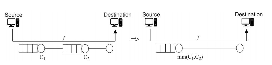 Figure 2‑51: Approximation of
a network using bottleneck server technique.
Figure 2‑51: Approximation of
a network using bottleneck server technique.
It is a common and a useful technique to reduce a network into a bottleneck link (from the perspective of a flow(s)) to study throughput and queue buildup. For example, a network with two links (in series) can be approximated by a single link of capacity \(\min{(C1,\ C2)}\) as illustrated in Figure 2‑51. Such analysis is commonly known as bottleneck server analysis. Single server queueing models such as M/M/1, M/G/1, etc. can provide tremendous insights on the flow and network performance with the bottleneck server analysis.
Multiple Flow Scenario

Figure 2‑52: Two flows \(\mathbf{f}_{\mathbf{1}}\) and \(\mathbf{f}_{\mathbf{2}}\) passing through a link \(\mathbf{l}\) of capacity \(\mathbf{C}_{\mathbf{l}}\)
Consider a scenario where multiple flows compete for the network resources. Suppose that the flows interact at some link buffer/server, say \(l\ \hat{}\), and compete for capacity. In such scenarios, the link capacity \(C_{_{l}^{\hat{}}\ }\) is shared among the competing flows and it is quite possible that the link can become the bottleneck link for the flows (limiting throughput). Here again, the queue tends to increase with the combined input flow rate and will grow unbounded as the combined input flow rate matches or exceeds the bottleneck link capacity. A plausible bound of throughput in this case is (under nicer assumptions on the competing flows)
\[throughput = \frac{C_{l}^{\hat{}}}{\ number\ of\ flows\ competing\ for\ capacity\ at\ link\ _{l}^{\hat{}}\ }\ bps\]
NetSim Simulation Setup
Open NetSim and click on Experiments> Internetworks> Network Performance> Throughput and Bottleneck Server Analysis then click on the tile in the middle panel to load the example as shown in below Figure 2‑53.

Figure 2‑53: List of scenarios for the example of Throughput and Bottleneck Server Analysis
Part - 1: A Single Flow Scenarios
We will study a simple network setup with a single flow illustrated in Figure 2‑54 to review the definition of a bottleneck link and the maximum application throughput achievable in the network. An application process at Wired_Node_1 seeks to transfer data to an application process at Wired_Node_2. We consider a custom traffic generation process (at the application) that generates data packets of constant length (say, L bits) with i,i,d. inter-arrival times (say, with average inter-arrival time \(v\) seconds). The application traffic generation rate in this setup is \(\frac{L}{v}\) bits per second. We prefer to minimize the communication overheads and hence, will use UDP for data transfer between the application processes.
In this setup, we will vary the traffic generation rate by varying the average inter-arrival time \(v\) and review the average queue at the different links, packet loss rate and the application throughput.
Procedure
We will simulate the network setup illustrated in Figure 2‑54 with the configuration parameters listed in detail in Table 2‑25 to study the single flow scenario.
NetSim UI displays the configuration file corresponding to this experiment as shown below:

Figure 2‑54: Network set up for studying a single flow
The following set of procedures were done to generate this sample.
Step 1: Drop two wired nodes and two routers onto the simulation environment. The wired nodes and the routers are connected with wired links as shown in (See Figure 2‑54).
Step 2: Click on the 'Set Traffic' tab in the ribbon at the top and configure a custom application between two wired nodes. To set the application properties as shown in below figure, click on the created application, expand the property panel on the right, and set the transport protocol to UDP. In the Packet Size tab, select Distribution as CONSTANT and set the value to 1460 bytes. In the Inter-Arrival Time tab, select Distribution as EXPONENTIAL and set the mean to 11680 microseconds.
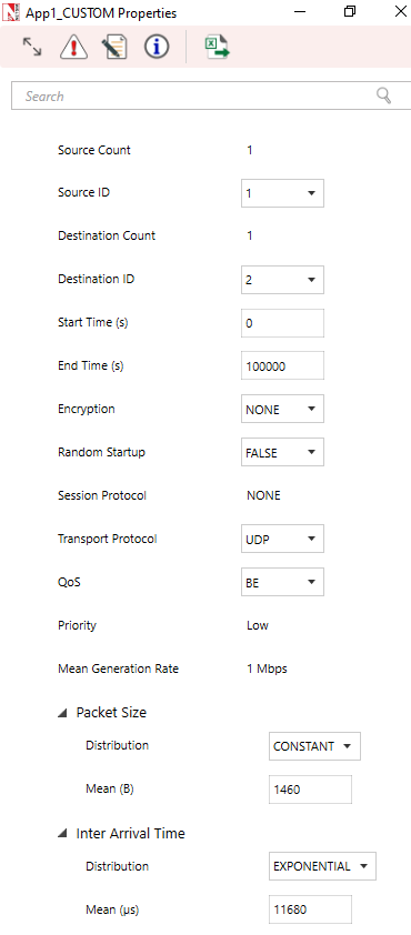
Figure 2‑55: Application configuration window
Step 3: The properties of the wired nodes are left to the default values.
Step 4: Click the link ID (of a wired link) and expand the property panel on right (see Figure 2‑56). Set Max Uplink Speed and Max Downlink Speed to 10 Mbps for link 2 (the backbone link connecting the routers) and 1000 Mbps for links 1 and 3 (the access link connecting the Wired Nodes and the routers).
Set Uplink BER and Downlink BER as 0 for links 1, 2 and 3. Set Uplink Propagation Delay and Downlink Propagation Delay as 0 microseconds for the two-access links 1 and 3 and 100 microseconds for the backbone link 2.

Figure 2‑56: Link Properties window
Step 5: Click on Router 3, expand the property panel on right and set the Buffer size to 8 MB in network layer of Interface 2 (WAN) as shown in Figure 2‑57.

Figure 2‑57: Router Properties window
Step 6: Click on Configure reports tab in ribbon on the top and enable packet trace. Packet Trace can be used for packet level analysis.
Step 7: Click on Run icon to access the Run Simulation window (see Figure 2‑58) and set the Simulation Time to 100 seconds and click on Run.

Figure 2‑58: Run Simulation window
Step 8: Now, repeat the simulation with different average inter-arrival times (such as 5840 µs, 3893 µs, 2920 µs, 2336 µs and so on). We vary the input flow rate by varying the average inter-arrival time. This should permit us to identify the bottleneck link and the maximum achievable throughput.
The detailed list of network configuration parameters is presented in (See Table 2‑25).
| Parameter | Value |
|---|---|
| LINK PARAMETERS | |
| Wired Link Speed (access link) | 1000 Mbps |
| Wired Link Speed (backbone link) | 10 Mbps |
| Wired Link BER | 0 |
| Wired Link Propagation Delay (access link) | 0 |
| Wired Link Propagation Delay (backbone link) | 100 µs |
| APPLICATION PARAMETERS | |
| Application | Custom |
| Source ID | 1 |
| Destination ID | 2 |
| Transport Protocol | UDP |
| Packet Size – Value | 1460 bytes |
| Packet Size – Distribution | Constant |
| Inter Arrival Time – Mean | AIAT (µs) |
| Inter Arrival Time – Distribution | Exponential |
| ROUTER PARAMETERS | |
| Buffer Size | 8 |
| MISCELLANEOUS | |
| Simulation Time | 100 Sec |
| Packet Trace | Enabled |
Table 2‑25: Detailed Network Parameters
Performance Measure
In Table 2‑26, we report the flow average inter-arrival time v and the corresponding application traffic generation rate, input flow rate (at the physical layer), average queue at the three buffers (of Wired Node 1, Router 3 and Router 4), average throughput (over the simulation time) and packet loss rate (computed at the destination).
Given the average inter-arrival time v and the application payload size L bits (here, 1460×8 = 11680 bits), we have,
\[Traffic\ generation\ rate = \frac{L}{v} = \frac{11680}{v}bps\]
\[input\ flow\ rate = \frac{11680 + 54*8}{v} = \frac{12112}{v}bps\]
where the packet overheads of 54 bytes is computed as \(54 = 8(UDP\ header) + 20(IP\ header) + 26(MAC + PHY\ header)\ bytes\). Let \(Q_{l}(u)\) as denote the instantaneous queue at link \(l\) at time \(u\) . Then, the average queue at link \(l\) is computed as
\[average\ queue\ at\ link\ l = \frac{1}{T}\int_{0}^{T}{Q_{l\ \ }(u)}\ \ du\ bits\]
where, \(T\) is the simulation time. The average throughput of the flow is computed as
\[throughput = \frac{application\ byte\ transferred}{T}bps\]
The packet loss rate is defined as the fraction of application data lost (here, due to buffer overflow at the bottleneck server).
\[packet\ loss\ rate\mathbf{=}\frac{application\ bytes\ not\ received\ at\ destination}{application\ bytes\ transmitted\ at\ source}\mathbf{\ }\]
Average Queue Computation from Packet Trace
Open Packet Trace from the Simulation Results window as shown below

Figure 2‑59: Opening Packet trace from Simulation results window
In packet trace, click on Insert on Top ribbon \(\rightarrow\) Select Pivot Table as shown in below figure
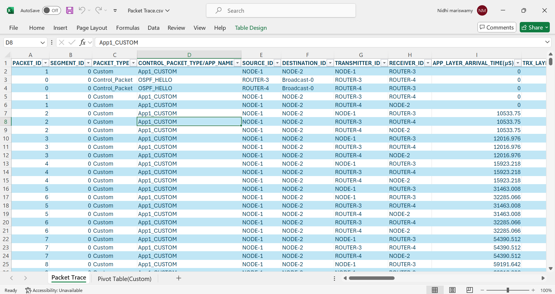
Figure 2‑60: Creating pivot table from packet trace
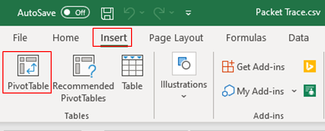
Figure 2‑61: Top Ribbon
The packet trace will be selected and Table 1 is mentioned as defualt, just click on OK.

Figure 2‑62: Packet Trace Pivot Table
Then we will get blank Pivot table.

Figure 2‑63: Blank Pivot Table
Packet ID drag and drop into Values field for 2 times, CONTROL PACKET TYPE or APP NAME, TRANSMITTER ID, RECEIVER ID into Filter field, NW LAYER ARRIVAL TIME (US) to Rows field see Figure 2‑64.
Change Sum of PACKET ID -> Values Field Settings ->Select Count -> ok for both Values field, CONTROL PACKET TYPE to APP1 CUSTOM, TRANSMITTER ID to Router 3 and RECEIVER ID to Router 4
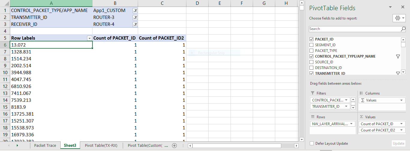
Figure 2‑64: Adding fields into Filter, Columns, Rows and Values
Right click on first value of Row Labels ->Group ->Select By value as 1000000.
Go to Values field under left click on Count of PACKET ID2 ->Values Field Settings-> click on show values as -> Running total in-> click on OK.
Again, create one more Pivot Table, Click on Insert on Top ribbon \(\rightarrow\) Select Pivot Table.
Then select packet trace and press Ctrl + A\(\ \ \rightarrow\) Select ok
Then we will get blank Pivot table see Figure 2‑65.
Packet ID drag and drop into Values field for 2 times,
CONTROL PACKET TYPE/APP NAME, TRANSMITTER ID, RECEIVER ID into Filter field, PHY LAYER ARRIVAL TIME (US) to Rows field see Figure 2‑65,
Change Sum of PACKET ID -> Values Field Settings ->Select Count -> ok for both Values field, CONTROL PACKET TYPE to APP1 CUSTOM, TRANSMITTER ID to Router 3 and RECEIVER ID to Router 4
Right click on first value of Row Labels for second Pivot Table->Group ->Select by value as 1000000.

Figure 2‑65: Create one more Pivot Table and Add All Fields
Go to Values field under left click on Count of PACKET ID ->Values Field Settings-> click on show values as -> Running total in-> click on OK.
Calculate the average queue by taking the mean of the number of packets in queue at every time interval during the simulation.
The difference between the count of PACKET ID2 (Column C) and count of PACKET ID2 (Column G), Note down the average value for difference see Figure 2‑66

Figure 2‑66: Average Packets in Queue
\[\mathbf{Packet\ Loss\ Rate\ (in\ percent)}\mathbf{=}\frac{\mathbf{Packet\ Generated - Packet\ Received}}{\mathbf{Packet\ Generated}}\mathbf{\times 100}\]
Results
In Table 2‑26, we report the flow average inter-arrival time (AIAT) and the corresponding application traffic generation rate (TGR), input flow rate, average queue at the three buffers (of Wired Node 1, Router 3 and Router 4), average throughput and packet loss rate.
AIAT \[\mathbf{v}\] (in µs) |
TGR \[\frac{\mathbf{L}}{\mathbf{v}}\] (in Mbps) |
Input Flow Rate (in Mbps) |
Average queue (in pkts) | Average Throughput (in Mbps) | Packet Loss Rate (in percent) | ||
|---|---|---|---|---|---|---|---|
Wired Node1 (Link 1) |
Router 3 (Link 2) |
Router4 (Link 3) |
|||||
| 11680 | 1 | 1.037 | 0 | 0 | 0 | 0.999925 | 0 |
| 5840 | 2 | 2.074 | 0 | 0.02 | 0 | 1.998214 | 0 |
| 3893 | 3.0003 | 3.1112 | 0 | 0.04 | 0 | 2.999307 | 0 |
| 2920 | 4 | 4.1479 | 0 | 0.11 | 0 | 3.996429 | 0 |
| 2336 | 5 | 5.1849 | 0 | 0.32 | 0 | 5.010136 | 0 |
| 1947 | 5.999 | 6.2209 | 0 | 0.4 | 0 | 6.000016 | 0.01 |
| 1669 | 6.9982 | 7.257 | 0 | 0.92 | 0 | 7.004496 | 0 |
| 1460 | 8 | 8.2959 | 0 | 2.05 | 0 | 8.028482 | 0 |
| 1298 | 8.9985 | 9.3313 | 0 | 5.43 | 0 | 9.009952 | 0.01 |
| 1284 | 9.0966 | 9.433 | 0 | 6.78 | 0 | 9.106429 | 0.01 |
| 1270 | 9.1969 | 9.537 | 0 | 7.78 | 0 | 9.208629 | 0.01 |
| 1256 | 9.2994 | 9.6433 | 0 | 7.81 | 0 | 9.313515 | 0 |
| 1243 | 9.3966 | 9.7442 | 0 | 11.32 | 0 | 9.416299 | 0.01 |
| 1229 | 9.5037 | 9.8552 | 0 | 16.21 | 0 | 9.52247 | 0.02 |
| 1217 | 9.5974 | 9.9523 | 0 | 25.89 | 0 | 9.614626 | 0.01 |
| 1204 | 9.701 | 10.0598 | 0 | 42.88 | 0 | 9.71811 | 0.05 |
| 1192 | 9.7987 | 10.1611 | 0 | 93.19 | 0 | 9.79695 | 0.26 |
| 1180 | 9.8983 | 10.2644 | 0 | 445.40 | 0 | 9.807696 | 1.15 |
| 1168 | 10 | 10.3699 | 0 | 856.25 | 0 | 9.808981 | 2.09 |
| 1062 | 10.9981 | 11.4049 | 0 | 3989.11 | 0 | 9.811667 | 11.00 |
| 973 | 12.0041 | 12.4481 | 0 | 4752.38 | 0 | 9.811667 | 18.53 |
| 898 | 13.0067 | 13.4878 | 0 | 5035.80 | 0 | 9.811667 | 24.75 |
| 834 | 14.0048 | 14.5228 | 0 | 5185.92 | 0 | 9.811667 | 30.09 |
| 779 | 14.9936 | 15.5481 | 0 | 5275.58 | 0 | 9.811667 | 34.75 |
Table 2‑26: Average queue, throughput and loss rate as a function of traffic generation rate.
We can infer the following from Table 2‑26,
The input flow rate is slightly larger than the application traffic generation rate. This is due to the overheads in communication.
There is queue buildup at Router 3 (Link 2) as the input flow rate increases. So, Link 2 is the bottleneck link for the flow.
As the input flow rate increases, the average queue increases at the (bottleneck) server at Router 3. The traffic generation rate matches the application throughput (with nearly zero packet loss rate) when the input flow rate is less than the capacity of the link.
As the input flow rate reaches or exceeds the link capacity, the average queue at the (bottleneck) server at Router 3 increases unbounded (limited by the buffer size) and the packet loss rate increases as well.
For the sake of the readers, we have made the following plots for clarity. In Figure 2 60, we plot application throughput as a function of the traffic generation rate. We note that the application throughput saturates as the traffic generate rate (in fact, the input flow rate) gets closer to the link capacity. The maximum application throughput achievable in the setup is 9.81 Mbps (for a bottleneck link with capacity 10 Mbps).
Figure 2‑67: Application throughput as a function of the traffic generation rate.
Figure 2‑64, we plot the queue evolution at the buffers of Links 1 and 2 for two different input flow rates. We note that the buffer occupancy is a stochastic process and is a function of the input flow rate and the link capacity as well.
At Wired Node 1 for TGR = 8 Mbps b) At Router 3 for TGR = 8 Mbps
At Wired Node 1 for TGR = 9.5037 Mbps d) At Router 3 for TGR = 9.5037 Mbps
Figure 2‑68: Queue evolution at Wired Node 1 (Link 1) and Router 3 (Link 2) for two different traffic generation rates
In Figure 2‑69, we plot the average queue at the bottleneck link 2 (at Router 3) as a function of the traffic generation rate. We note that the average queue increases gradually before it increases unboundedly near the link capacity.
Figure 2‑69: Average queue (in packets) at the bottleneck link 2 (at Router 3) as a function of the traffic generation rate
Bottleneck Server Analysis as M/G/1 Queue
Let us now analyze the network by focusing on the flow and the bottleneck link (Link 2). Consider a single flow (with average inter-arrival time v) into a bottleneck link (with capacity C). Let us the denote the input flow rate in packet arrivals per second as \(\lambda\) , where \(\lambda = 1/\ v\) . Let us also denote the service rate of the bottleneck server in packets served per second as \(\mu\), where \(\mu = \frac{C}{L + 54 \times 8}\) . Then,
\[\rho = \ \lambda \times \frac{1}{\mu} = \frac{\lambda}{\mu}\]
denotes the offered load to the server. When \(\rho < 1\), \(\rho\) also denotes (approximately) the fraction of time the server is busy serving packets (i.e., \(\rho\)denotes link utilization). When \(\rho \ll 1\), then the link is barely utilized. When \(\rho > 1\), then the link is said to be overloaded or saturated (and the buffer will grow unbounded). The interesting regime is when \(0 < \rho < 1\).
Suppose that the application packet inter-arrival time is i.i.d. with exponential distribution. From the M/G/1 queue analysis (in fact, M/D/1 queue analysis), we know that the average queue at the link buffer (assuming large buffer size) must be.
\[average\ queue = \ \rho \times \frac{1}{2}\left( \frac{\rho^{2}}{1 - \rho} \right),\ \ 0\ < \ \rho\ < \ 1\]
where, \(\rho\) is the offered load. In Figure 2‑69, we also plot the average queue from (1) (from the bottleneck analysis) and compare it with the average queue from the simulation. You will notice that the bottleneck link analysis predicts the average queue (from simulation) very well.
An interesting fact is that the average queue depends on \(\ \lambda\) and \(\mu\) only as \(\rho = \frac{\ \lambda}{\mu}\).
Part - 2: Two Flow Scenario
We will consider a simple network setup with two flows illustrated in Figure 2‑70 to review the definition of a bottleneck link and the maximum application throughput achievable in the network. An application process at Wired Node 1 seeks to transfer data to an application process at Wired Node 2. Also, an application process at Wired Node 3 seeks to transfer data to an application process at Wired Node 4. The two flows interact at the buffer of Router_ 5 (Link 3) and compete for link capacity. We will again consider custom traffic generation process (at the application processes) that generates data packets of constant length (L bits) with i.i.d. inter-arrival times (with average inter-arrival time \(v\) seconds) with a common distribution. The application traffic generation rate in this setup is \(\frac{L}{v}\) bits per second (for either application).
In this setup, we will vary the traffic generation rate of the two sources (by identically varying the average inter-arrival time v) and review the average queue at the different links, application throughput (s) and packet loss rate (s).
Procedure
We will simulate the network setup illustrated in Figure 2‑70 with the configuration parameters listed in detail in Table 2‑25 to study the two-flow scenario. We will assume identical configuration parameters for the access links and the two application processes.

Figure 2‑70: Network set up for studying two flows
Step 1: Right-click the link ID (of a wired link) and select Properties to access the link’s properties window. Set Max Uplink Speed and Max Downlink Speed to 10 Mbps for link 3 (the backbone link connecting the routers) and 1000 Mbps for links 1,2,4, 5 (the access link connecting the Wired Nodes and the routers). Set Uplink BER and Downlink BER as 0 for all links. Set Uplink Propagation Delay and Downlink Propagation Delay as 0 microseconds for links 1,2,4 and 5 and 100 microseconds for the backbone link 3.
Step 2: Enable Packet trace in NetSim GUI.
Step 3: Simulation time is 100 sec for all samples.
Results
In Table 2‑27, we report the common flow average inter-arrival time (AIAT) and the corresponding application traffic generation rate (TGR), input flow rate, combined input flow rate, average queue at the buffers (of Wired Node 1, Wired Node 3 and Router 5), average throughput(s) and packet loss rate(s).
AIAT \(\mathbf{v}\) (in µs) |
TGR \[\frac{\mathbf{L}}{\mathbf{v}}\] (in Mbps) |
Input Flow Rate (in Mbps) |
Combined Input Flow Rate (in Mbps) | Average queue (In pkts) |
Average Throughput (in Mbps) |
Packet Loss Rate (In percent) |
||||
|---|---|---|---|---|---|---|---|---|---|---|
| WN1 | WN2 | Router | App1 | App2 | App1 | App2 | ||||
| 11680 | 1.000 | 1.037 | 2.074 | 0 | 0 | 0.03 | 0.999 | 1.002 | 0 | 0 |
| 5840 | 2.000 | 2.074 | 4.148 | 0 | 0 | 0.16 | 1.998 | 2.006 | 0 | 0 |
| 3893 | 3.000 | 3.111 | 6.222 | 0 | 0 | 0.32 | 2.999 | 3.001 | 0 | 0 |
| 2920 | 4.000 | 4.147 | 8.295 | 0 | 0 | 1.94 | 3.996 | 4.018 | 0 | 0 |
| 2336 | 5.000 | 5.184 | 10.369 | 0 | 0 | 852.73 | 4.903 | 4.907 | 2.12 | 2.10 |
| 1947 | 5.999 | 6.220 | 12.441 | 0 | 0 | 4767.77 | 4.895 | 4.917 | 18.42 | 18.35 |
| 1669 | 6.998 | 7.257 | 14.514 | 0 | 0 | 5195.27 | 4.884 | 4.928 | 30.27 | 29.82 |
| 1460 | 8.000 | 8.295 | 16.591 | 0 | 0 | 5345.82 | 4.903 | 4.908 | 38.92 | 38.75 |
| 1298 | 8.998 | 9.331 | 18.662 | 0 | 0 | 5422.26 | 4.907 | 4.904 | 45.53 | 45.55 |
| 1168 | 10 | 10.369 | 20.738 | 0 | 0 | 5468.07 | 4.919 | 4.892 | 50.90 | 51.15 |
Table 2‑27: Average queue, throughput(s) packet loss rate(s) as a function of the traffic generation
We can infer the following.
There is queue buildup at Router 5 (Link 3) as the combined input flow rate increases. So, link 3 is the bottleneck link for the two flows.
The traffic generation rate matches the application throughput(s) (with nearly zero packet loss rate) when the combined input flow rate is less than the capacity of the bottleneck link.
As the combined input flow rate reaches or exceeds the bottleneck link capacity, the average queue at the (bottleneck) server at Router 5 increases unbounded (limited by the buffer size) and the packet loss rate increases as well.
The two flows share the available link capacity and see a maximum application throughput of 4.9 Mbps (half of bottleneck link capacity 10 Mbps).
Useful Exercises
Redo the single flow experiment with constant inter-arrival time for the application process. Comment on average queue evolution and maximum throughput at the links.
Redo the single flow experiment with small buffer size (8 KBytes) at the bottleneck link 2. Compute the average queue evolution at the bottleneck link and the average throughput of the flow as a function of traffic generation rate. Compare it with the case when the buffer size in 8 MB.
Redo the single flow experiment with a bottleneck link capacity of 100 Mbps. Evaluate the average queue as a function of the traffic generation rate. Now, plot the average queue as a function of the offered load and compare it with the case of bottleneck link with 10 Mbps capacity (studied in the report).