Simulation GUI
Open NetSim, Go to New Simulation 🡪 Satellite Comm. Networks
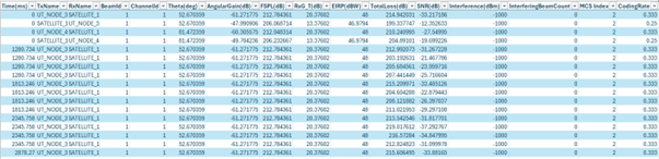
Figure-1: NetSim Home Screen
Create Scenario
Satellite Communication Networks palette features various devices like Wired Nodes, L2 Switch, Access Point, Wireless node, UT Router (User Terminal Router), Router, UT Node (User Terminal Node), Satellite Gateway, and Satellite.
Devices specific to NetSim Satellite Comm. Library
UT - User Terminal. The user terminals are part of the same communication network as the Satellite Gateway. The User Terminals in NetSim are UT Node and UT Router
UT Router - User Terminal Router. A UT Router is used when a separate communication network is required. The typical use case is where there are multiple devices downstream who seek to utilize the sat-com link. The UT Router cannot be a source of any traffic.
Satellite Gateway: Each gateway has two interfaces, a satellite interface and multiple wired interfaces. The satellite interface connects via the forward link to the satellite. The wired interface allows for connection to routers via the wired interface. When connected to a satellite, the user terminals mapped to the gateway are part of the same network. Multiple gateways can be configured per satellite, and round-robin scheduling is run (at the Network control center (NCC) which is not displayed in NetSim GUI)
Satellite: Since the satellite model is a bent pipe and satellite does not have an IP. NetSim supports single satellite communication, and it can be connected to multiple gateways and to multiple user terminals. The satellite node cannot be the source of any traffic. The default altitude of the Satellite is 35,768,000 meters, which represents the circular geosynchronous orbit.
Coordinate System: NetSim uses a Geodetic co-ordinate system. The altitude is from Mean Sea level. The geocentric co-ordinate system uses distance from the centre of the earth.
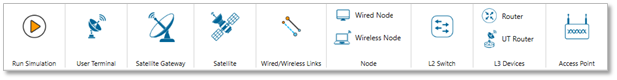
Figure-2: The devices present in the ribbon in NetSim’s GUI
Placement of devices on the grid environment
Add a User Terminal (UT) – Click the User Terminal > UT Node icon on the toolbar and place the device in the grid. UT Node must be connected to Satellite.
Add a UT Router – Click the User Terminal > UT Router icon on the toolbar and place the device in the grid. UT Router must be connected to a Node or to a L2 Switch or to a Router or to an Access_Point or Satellite.
Add a Satellite – Click the Satellite icon on the toolbar and place the Satellite in the grid. Satellite must be connected to a Satellite Gateway or to a UT Node or to a UT Router.
Add a Satellite Gateway – Click the Satellite Gateway icon on the toolbar and place the Satellite Gateway in the grid. Satellite Gateway must be connected to a Satellite or to a Router.
Add a Router – Click the Router icon on the toolbar and place the Router in the grid.
Add a Wired Node – Click the Wired Node icon on the toolbar and place the device in the grid.
Add a L2 Switch – Click the L2 Switch icon on the toolbar and place the device in the grid.
Add an Access Point – Click the Access Point icon on the toolbar and place the Access Point in the grid.
Add a Wireless Node – Click the Wireless Node icon on the toolbar and place the device in the grid.
Enable Packet Trace, Event Trace (Optional)
Click Packet Trace / Event Trace icon in the Configure Reports option and check Enable Packet Trace / Event Trace check box. For detailed help about the packet and event trace, please refer to sections 8.4 and 8.5 in the User Manual.
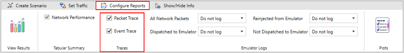
Figure-3: Enable Packet Trace, Event Trace & Plots options on top ribbon
Enable protocol specific logs and plots
NetSim provides protocol-specific logs for Satellite libraries, which users can enable before running a simulation. These can be enabled by clicking on configure reports in top ribbon > clicking on plots > choosing as desired, and running the simulation.
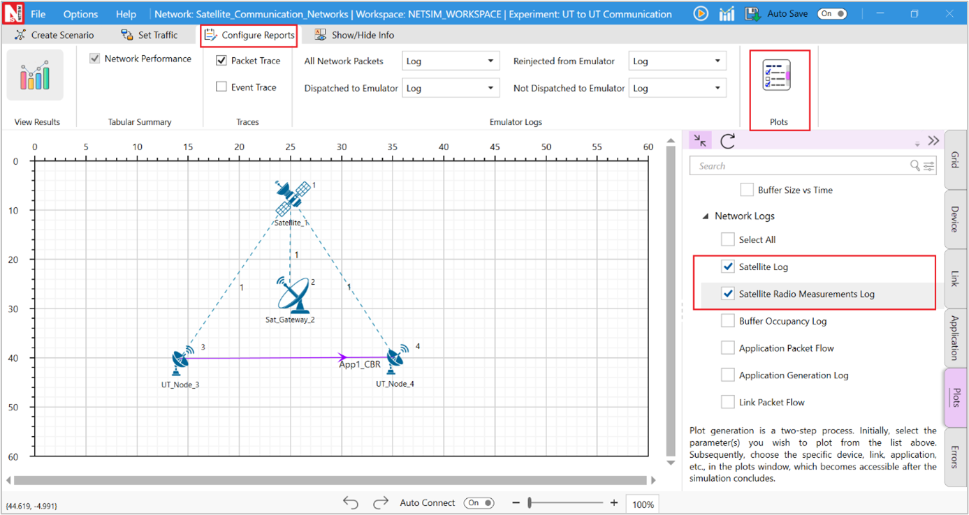
Figure-4: Enabling the Network logs in Satellite network
Similarly, users can enable the plots for Satellite Radio Measurements.
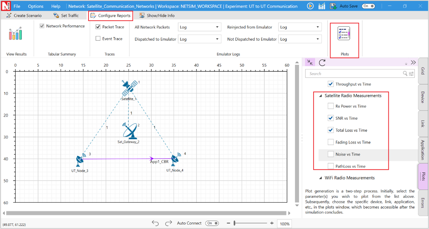
Figure-5: Enabling the Plots in Satellite
GUI Configuration Parameters
The SATELLITE parameters can be accessed by right clicking on a Satellite, Satellite Gateway, UT Router or UT and selecting Interface (SATELLITE) Properties 🡪 Datalink and Physical Layers.
Satellite Properties |
||||
|---|---|---|---|---|
Interface (Satellite) – Physical Layer |
||||
Parameter |
Type |
Range |
Description |
|
G/T (dBk) |
Local |
0-100000dBk |
Antenna gain-to-noise-temperature is (G/T) where G is the antenna gain in decibels at the receive frequency, and T is the equivalent noise temperature of the receiving system in kelvins. |
|
Tx Power |
Local |
-10000dBW to 10000dBW |
It is the signal intensity of the transmitter. The higher the power radiated by the transmitter's antenna the greater the reliability of the communications system. |
|
Access Protocol |
Fixed |
TDMA |
TDMA allows a number of clients to access a single radio-frequency channel without interference by allocating unique time slots to each user within each channel, reducing the loss of packets and improving the data rate thereby delivering QoS to the clients. |
|
Fixed |
MF-TDMA |
Multi-frequency time-division multiple access is a technology for dynamically sharing bandwidth resources in an over-the-air two-way communications network. |
||
Base Frequency (GHz) |
Local |
Ku-band: 12-18GHz Ka-band: 26-40GHz |
The “band” in use refers to the radio frequencies used to and from the satellite: Ku-band services uses the 12 - 18 GHz, and Ka-band services uses the 26- 40 GHz segment of the electromagnetic spectrum |
|
Band |
Fixed |
KU |
Microwave frequency band used for satellite communication and broadcasting, using frequencies in the range of 12 -18 GHz |
|
Fixed |
KA |
Microwave frequency band used for satellite communication and broadcasting, using frequencies in the range of 26 - 40 GHz |
||
Rolloff Factor |
Local |
0-1 |
In NetSim, Symbol Rate = BW / (1+Roll of factor) and Bit Rate = Symbol rate * Modulation order * CodeRate |
|
Spacing Factor |
Local |
0-1 |
In NetSim EffectiveBandwidth (Hz) = AllocatedBandwidth (Hz) / ((RollOffFactor + 1.0) * (SpacingFactor + 1.0)); Spacing factor should be in the range of [0,1] |
|
Carrier Bandwidth (Hz) |
Local |
0-1000000 Hz |
Bandwidth of the carrier in Hz |
|
Framecount in Superframe |
Local |
0-1000000 |
Number of frames present in a superframe. |
|
Frame Bandwidth (Hz) |
Local |
0-1000000 Hz |
Bandwidth of the frame in Hz. |
|
Frame Usage Mode |
Local |
NORMAL SHORT |
Baseband frame usage modes. |
|
Modulation |
Local |
QPSK 8PSK 16APSK 16QAM 32APSK |
Modulation is the process of varying one waveform in relation to another waveform. It is used to transfer data over an analog channel. |
|
Coding Rate |
Local |
1/3,1/2, 3/5, 2/3, 3/4, 4/5, 5/6, 8/9, 9/10 |
It states what portion of the total amount of information that is useful(non-redundant). This code rate typically a fractional number. |
|
S**lot Count in Frame |
Local |
Short Frame: QPSK-90, 8PSK-60, 16APSK/16QAM-45, 32APSK-36 Normal Frame: QPSK-360, 8PSK-240, 16APSK/16QAM-180, 32APSK-144 |
The number of slots per frame. The number of slots per frame is based on modulation and frame type chosen. |
|
Symbol per Slot |
Local |
0-1000000 |
The number of TDMA symbols within a slot, the default value of symbol per slot is 90. |
|
Pilot Block Size (Symbols) |
Local |
0-1000000 symbols |
Size of pilot block in symbols |
|
Pilot Block Interval (Slots) |
Local |
0-1000000 slots |
Interval (in symbols) between Pilot blocks |
|
Pilot Header (Slots) |
Local |
0-1000000 slots |
The pilot block header size in slots. |
|
Frame Header Length (Bytes) |
Local |
0-1000000 bytes |
Baseband frame header length in bytes |
|
BER Model |
Local |
Fixed |
BER value is based on the user input and is independent of the received SINR. |
|
FILE BASED |
File Based is a feature in NetSim with which users can define the BER. Users will have to provide a BER_FILE.txt file as input to NetSim by clicking on the Open file link the Physical Layer-Properties of the device. |
|||
MODEL BASED |
BER is computed using the SINR-BER formula for the chosen Modulation and coding. The pathloss and fading models are used in the SINR calculation. |
|||
BER |
Local |
0.00000001-1 |
This parameter is shown is the Fixed option is chosen for the BER model parameter. Users can set the Bit Error Rate (BER) in the range shown. |
|
UT Properties |
||||
Interface (Satellite) – Physical Layer |
||||
Parameter |
Parameter |
Parameter |
Parameter |
|
Tx Antenna Gain (dB) |
Local |
0-1000000dB |
A relative measure of an antenna’s ability to direct or concentrate radio frequency energy in a particular direction or pattern at the transmitter side. |
|
Rx Antenna Gain (dB) |
Local |
0-1000000dB |
A relative measure of an antenna’s ability to receive radio frequency energy in a particular direction or pattern at the receiver side. |
|
Table-1: Satellite, Satellite Gateway, UT Router or UT and selecting Interface (SATELLITE) Properties 🡪 Physical Layers Description
Propagation Model |
||||
|---|---|---|---|---|
Link Properties |
||||
Parameter |
Type |
Range |
Description |
|
Propagation Medium |
Link |
Air |
Medium of propagation in NetSim would be Air for RF waves. |
|
Channel Characteristics |
Fixed |
Pathloss and Fading and Shadowing |
Path loss and fading and shadowing: In pathloss models, for a fixed distance between source and destination, path loss is same. We get varied path loss for some distance between source and destination in shadowing and fading is variation of the attenuation of a signal with various variables. These variables include time, geographical position, and radio frequency. |
|
Shadowing Model |
Fixed |
NONE |
||
Pathloss Model |
Link |
Friis Free Space |
It Used to model the LOS path loss incurred in the channel. the Friis Free space model is restricted to unobstructed clear path between the transmitter and the receiver. |
|
Pathloss Exponent (η) |
Fixed |
2 |
Path loss exponent indicates the rate at which the path loss increases with distance. The value depends on the specific propagation environment. |
|
Fading Model |
Fixed |
Markov Loo |
Each state of the three-state Markov channel models obeys the Loo distribution with different parameters; while the state transition is modeled as a first-order Markov random process. |
|
Direct Signal Mean (dB) |
Link |
-∞ to ∞ |
Mean value of the direct signal, value can be differentiated according to the state. |
|
Direct Signal Standard Dev (dB) |
Link |
0 to ∞ |
Standard Deviation of the direct signal value can be differentiated according to the state. |
|
RMS Multipath Power (dB) |
Link |
-∞ to ∞ |
RMS squared multipath power in dB |
|
Number of Direct Signal Oscillators |
Link |
0 to ∞ |
Number of direct signal oscillator is used for frequency conversion process in superheterodyne receiver. |
|
Number of Multipath Oscillators |
Link |
0 to ∞ |
Number of multipath oscillators is used to generate higher oscillation frequencies. |
|
Direct Signal Doppler (Hz) |
Link |
0 to ∞ |
||
Multipath Doppler (Hz) |
Link |
0 to ∞ |
The normalized PSD (its integral in the whole frequency range equals to one) constitutes the PDF for the Doppler frequencies, arising from the different angles of arrival the multipath components have with respect to the receiver’s motion. |
|
Initial Probability |
Link |
0 to 1 |
An initial probability distribution, defined on S, specifies the starting state. Usually this is done by specifying a particular state as the starting state. |
|
Table-2: Propagation Model/Wireless Link Properties Description
Mapping of User Terminal (UT Node / UT Router) to Satellite Gateway
Each satellite can be connected to multiple Satellite Gateways and to Multiple User Terminals. The following screen shot shows how to map the User Terminal to Satellite Gateway as shown Figure-6.
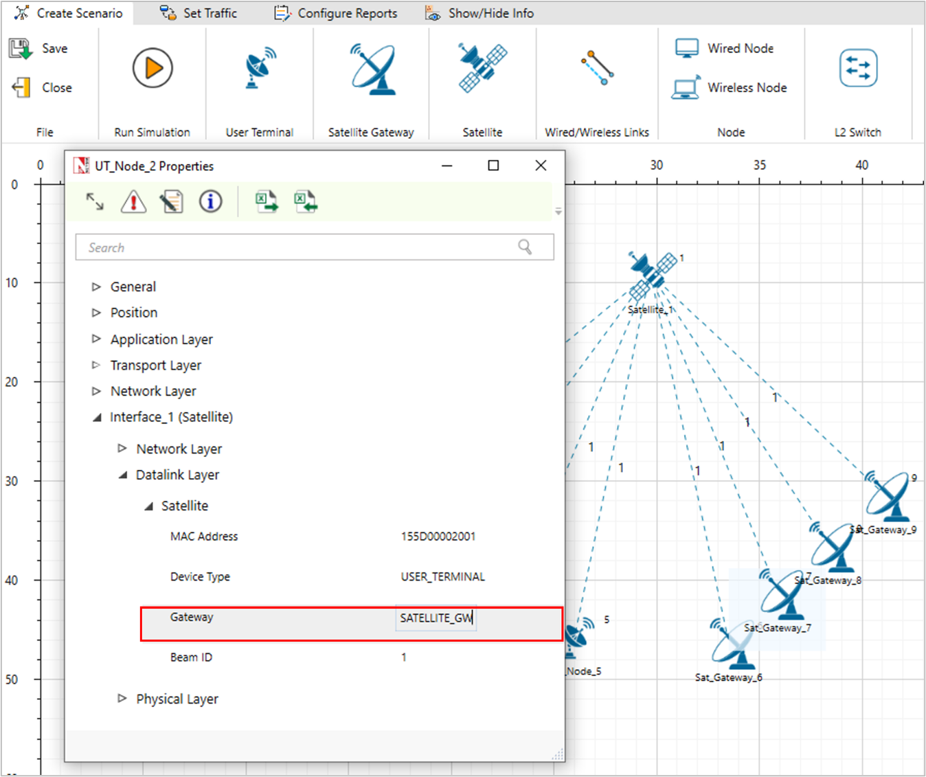
Figure-6: Mapping of User Terminal (UT Note / UT Router) to Satellite Gateway
In order to Map User Terminal (UT Node / UT Router) to Satellite Gateway right click go to the properties of UT Node/UT Router 🡪 INTERFACE1 (SATELLITE) 🡪 DATALINK LAYER 🡪 Gateway user can map the Satellite Gateway with UT Node / UT Router accordingly.
Additionally, in the UT Router/UT Node -> Interface Satellite the default gateway IP should be set as the IP of the connected Satellite Gateway.
Incorrect mapping of the Satellite Gateway and/or the default Gateway IP address, in the properties of the UT Node / UT Router could lead application crash or NIL application throughputs.
Configuring Static Routes
After mapping the UT Router/UT Node to a Satellite Gateway, static routes need to be configured in the devices to forward traffic. Let us consider the following network scenario as shown Figure-7.
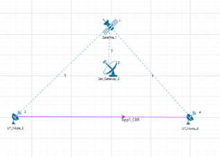
Figure-7: Network Topology in this experiment
In this network scenario, for UDP traffic to be sent from UT Node 3 to UT Node 4, static routes need to be set in UT Node 3 and in the Satellite Gateway 2.
If TCP traffic needs to be sent from UT Node 3 to UT Node 4, then static routes need to be set in UT Node 4 as well. This is essential for connection establishment and sending acknowledgements.
Refer the featured example on Configuring applications from UT Node to UT Node for detailed information on static route configuration.