Model Features
TDMA Forward Link and MF TDMA Return Link
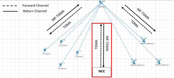
Figure-1: Forward and Return links. The Network Control Centre (NCC) is not displayed in NetSim and is assumed to be part of every satellite
In NetSim, a Forward link is defined as the direction from Satellite Gateway to Satellite to UT Node / UT Router. A Return link is defined as the direction from the UT Node / UT Router to Satellite to the Satellite Gateway.
The protocol operating in the Forward link is Time Division Multiple Access (TDMA). The protocol operating in the Return link is Multi Frequency Time Devision Multiple Access (MF-TDMA).
Both the Forward link and Return link transmissions in NetSim are modeled as Layer-2 transmissions. The framing is as explained in the subsequent paragraph.
Each Super Frame is composed of a number of Frames. This is taken as a user input, given by the attribute Framecount in SuperFrame available in Satellite -> Interface Satellite -> Physical Layer properties. The frames in turn are composed of carriers (in frequency) and slots (in symbols). The number of carriers would be
The number of slots per frame is determined by the modulation scheme chosen by the user.
Modulation and coding schemes supported
QPSK with coding rates 1/3, 1/2,1/4, 2/5, 3/5, 2/3, 3/4, 4/5, 5/6, 8/9, 9/10
8PSK with coding rates 3/5, 2/3, 3/4, 5/6, 8/9, 9/10
16APSK with coding rates 2/3, 3/4, 4/5, 5/6, 8/9, 9/10
16QAM with coding rates 3/4, 5/6
32APSK with coding rates 3/4, 4/5, 5/6, 8/9, 9/10
Note:
The modulation and coding rate are specified in Table 12 on page 32 of the ETSI EN 302 307-1 European Standard
Physical layer framing for forward and return links
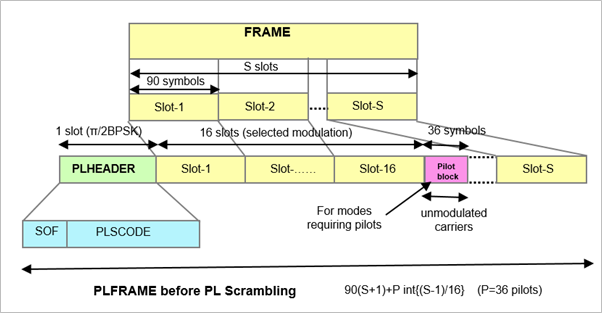
Figure-2: Format of a “Physical Layer Frame” PLFRAME
\[\mathbf{\eta}_{\mathbf{ldpc}}\mathbf{= 64800\ }\]
\[\mathbf{(normal\ frame)}\]
|
\[\mathbf{l = 16200\ }\]
\[\mathbf{(short\ frame)}\]
|
|||
|---|---|---|---|---|
\[\mathbf{\eta}_{\mathbf{MOD}}\mathbf{\ (bits/Hz)}\]
|
\[S\]
|
\[\eta\ \%\ no - pilot\]
|
\[S\]
|
\[\eta\ \%\ no - pilot\]
|
2 |
360 |
99.72 |
90 |
98.90 |
3 |
240 |
99.59 |
60 |
98.36 |
4 |
180 |
99.45 |
45 |
97.83 |
5 |
144 |
99.31 |
36 |
97.30 |
Table-1: S = number of SLOTs per FRAME (number of symbols per slot is 90)
The normal frame and short frame setting can be done using the Frame Usage Mode parameter in the GUI as shown Figure-3.
Changing the Modulation scheme in UI would change the value of S (Slot count in frame)
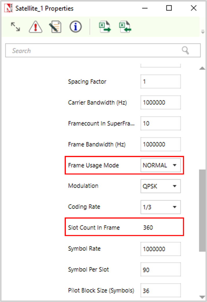
Figure-3: Satellite > Physical layer properties window
Default NetSim GUI settings
Symbols per slot: 90
Pilot Block size (symbols): 36
Pilot block interval (slots): 16
PL header size (slots): 1
Frame header size (In bytes): 10 (per ETSI EN 302 307 V1.3.1)
Frame Type: Normal (Options are normal or short)
Satellite PHY: Data Rate
Given below is the data rate calculation methodology for both forward and return links. The parameter values used are the default values in NetSim GUI.
The number of Modulation Bits depends on the modulation scheme per the table below:
Modulation |
Modulation bits |
|---|---|
QPSK |
2 |
8PSK |
3 |
16APSK/16QAM |
4 |
32APSK |
5 |
Table-2: Modulation bits for different modulation
Analytical throughput estimation
Let us an example in which the Packet Size (App layer) is 1460B which translates to 1488B at the PHY layer after addition of overheads, with QPSK modulation and \(\frac{1}{2}\) coding rate. For this modulation and coding rate the raw PhyRate of the channel is 162249 bps using the formulas given in 3.4. The analytical throughput estimate for such a scenario would be:
\(PacketsPerFrame\) is the number of packets that can be packed in a frame, and hence the greatest integer or floor function is used.
PHY rate for various modulations and coding rates
Modulation |
Modulation bits |
Slot Count in a frame |
Coding Rate |
PHY Rate (Mbps) |
|---|---|---|---|---|
QPSK |
2 |
360 |
1/3 |
0.167 |
1/2 |
0.250 |
|||
1/4 |
0.125 |
|||
2/5 |
0.200 |
|||
3/5 |
0.300 |
|||
2/3 |
0.333 |
|||
3/4 |
0.375 |
|||
4/5 |
0.400 |
|||
5/6 |
0.417 |
|||
8/9 |
0.444 |
|||
9/10 |
0.450 |
|||
8PSK |
3 |
240 |
3/5 |
0.450 |
2/3 |
0.500 |
|||
3/4 |
0.561 |
|||
5/6 |
0.625 |
|||
8/9 |
0.667 |
|||
9/10 |
0.675 |
|||
16APSK |
4 |
180 |
2/3 |
0.667 |
3/4 |
0.750 |
|||
4/5 |
0.800 |
|||
5/6 |
0.833 |
|||
8/9 |
0.889 |
|||
9/10 |
0.900 |
|||
16QAM |
4 |
180 |
3/4 |
0.750 |
5/6 |
0.833 |
|||
32APSK |
5 |
144 |
3/4 |
0.936 |
4/5 |
1.000 |
|||
5/6 |
1.042 |
|||
8/9 |
1.111 |
|||
9/10 |
1.125 |
|||
Table-3: List of support modulation schemes and coding rates, and their respective PHY Rates
Satellite PHY: Land Satellite Channel Model
Propagation
The distance between the ground nodes and the satellite determines the propagation delay and path loss of the radio signal. The distance is computed based on the cartesian distance between the ground nodes and the satellite. NetSim computes the propagation delay of the radio signal traveling from the source node to the destination node at the speed of light. The propagation model calculates the weakening of the radio signal as it propagates from the source node per the pathloss and fading model.
Pathloss Model – Friis Free Space Propagation
The free space propagation model is used to predict received signal strength when the transmitter and receiver have a clear, unobstructed line-of-sight path between them. Satellite communication systems and microwave line-of-sight radio links typically undergo free space propagation. The mathematical expression for free-space path loss is given by the Friis Free-Space Equation:
where \(P_{t}\)is the transmitted power.
\(P_{r}\) is the received power.
\(G_{t}\) is the transmitter antenna gain.
\(G_{r}\) is the receiver antenna gain.
d is the T-R separation distance in meters.
λ is the wavelength in meters.
Fading model
NetSim uses a 3 state (state 1, state 2 and state 3) Markov model to simulate fading.
The conditional probabilities of state \(s_{n + 1}\) given the state \(s_{n}\)are described by state transition probabilities \(p_{ij}\)
Where \(S_{1}\), \(S_{2}\), \(S_{3}\) denotes respective channel state, \(P_{ij}\) is the probability the Markov process goes from state i to state j.
Figure-4: Switching of three-state Markov process
The switching among each state is described by a transition matrix P, which is
Each state of the three-states of the Markov model obeys the Loo distribution with different parameters, while the state transition is modeled as a first-order Markov random process.
The Loo distribution considers the received signal as a sum of two signal components. A log-normally distributed direct signal expresses the slow fading component corresponding to varying shadowing conditions of the direct signal. A Rice distribution characterizes the fast-fading component due to multipath effects.
The Loo parameter triplet consists of the mean, the standard deviation for the log-normally distributed direct signal, and the average multipath power.
Depending on the current state interval and on the environment of the terminal, a new random Loo parameter triplet is generated. The output of the channel model is a time-series of the received signal in form of a complex envelope.
And finally, the model computes the Loo distributed time-series including Doppler shaping for every new state interval, which is the output of the proposed LMS channel model.
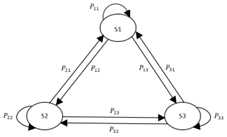
Figure-5: The Satellite LMS channel Model
SNR - BER Calculation
The SNR is calculated separately for each ‘hop’ of each link. This means the calculation is done from Gateway to Satellite and then separately again from Satellite to UT, and vice versa.
\(Noise = k_{B}\ T\ B\) where \(k_{B}\)is the Boltzman’s constant, B is the carrier bandwidth and \(T\) is the temperature calculated per user input of \(\frac{G}{T}(dBK)\ \)in NetSim UI.
NetSim provides three options for BER.
Model Based: The BER is then calculated for each link based on the SNR. Please see Propagation-Models.pdf document for detailed information on BER calculation.
Fixed: the BER value can be input in the GUI. If this option is chosen, the SNR (derived from propagation model) is not used.
File Based: SNR – BER table should be provided in a file per the format given below. This table should be in increasing order of SNR. The SNR is calculated by NetSim from the RF propagation model. For this SNR, the appropriate BER is selected from this table. BER is 1.0 for any SNR value below SNR1, and BER is 0.0 for any SNR greater than SNRn.
SNR1, BER1
SNR2, BER2
…
SNRn, BERn
Note: Users can enable the Satellite Propagation Log to see the SNR calculated from RF propagation model and then choose appropriate entries of SNR, BER values into the BER-File to see the impact on throughput.
Results
Please refer NetSim User manual section 8 for Results and Analysis.
Satellite Log
NetSim Satellite Log file records UT Satellite association, calculated superframe, frame, slot, bandwidth, etc., This log can be enabled/disabled by going to Plots option and checking/unchecking the Satellite Log option under the Network Logs section as shown below:
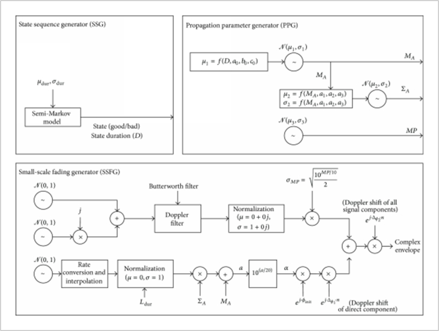
Figure-6: Enabling Satellite Log file.
A log file specific to satellite communication, is generated post simulation as shown in screen shot below,
Figure-7: Result Window
On opening, the satellite log file would look like the image below.
Figure-8: NetSim Satellite communication log file
This file logs details such as
UT – Satellite Gateway association
Calculated Super frame, frame, slot, bandwidth, carrier count etc. for each satellite.
Frame by frame transmissions with time stamps
Satellite Radio Measurements Log
NetSim Satellite Radio Measurements Log file records Time (ms), Transmitter name, Receiver name, Slant height(km), EIRP (dBW), Elevation Angle(\({^\circ}\)), RXG_T, Pathloss(dB),Fading loss(dB), Additional loss(dB), Total loss(dB), Angular gain( dB), Rx power (dBm), SNR (dB), Thermal noise(dBm), Channel Id, Beam Id, MCS Index and Coding rate. This log can be enabled/disabled by going to Logs option and checking/unchecking the Satellite Radio Measurements Log option under the Network Logs section as shown below:
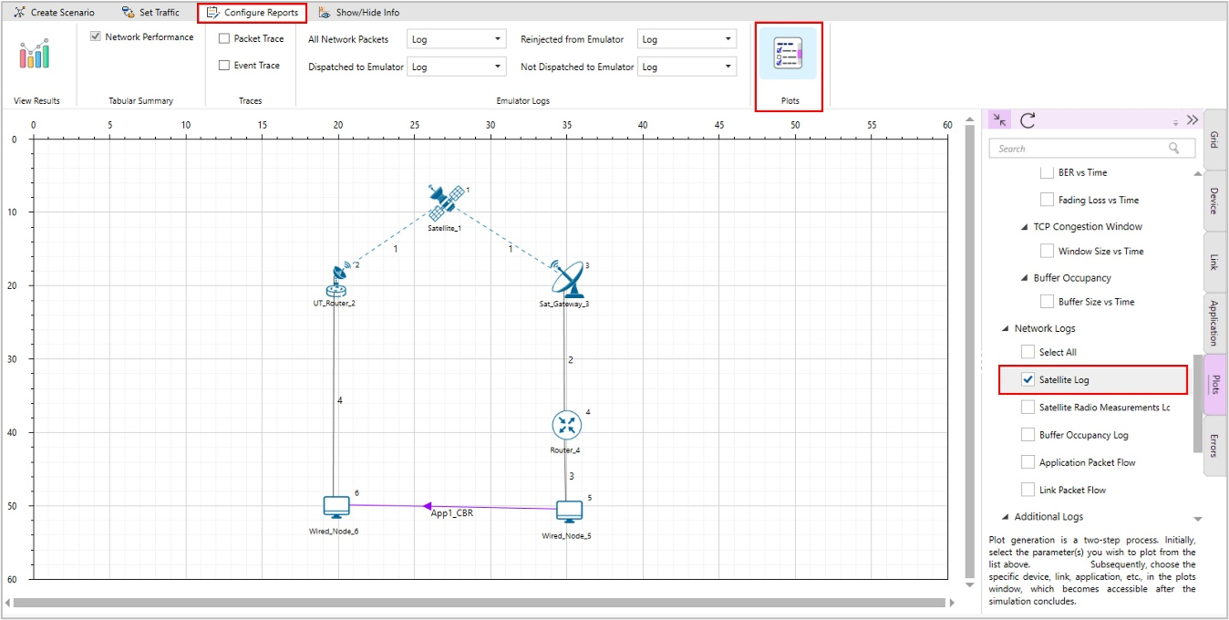
Figure-9: Enabling Satellite Radio Measurements Log file.
The Satellite Radio Measurements.csv file will contain the following information:
Time in Milliseconds
Transmitter Name
Receiver Name
Transmitter Power in dBm
Pathloss in dB
Shadowing Loss in dB
Fading Loss in dB
Total Loss in dB
Received Power in dBm
Noise in dBm
SNR in dB
Satellite Radio Measurements log files will be available under the Logs in the results window as shown below:
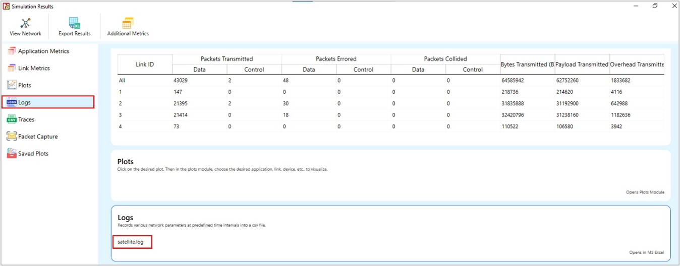
Figure-10: Result Window
Users can see Tx Power, Rx power, pathloss, fading-loss, Total loss, Thermal noise, and SNR values in the Log files for each forward and return link.
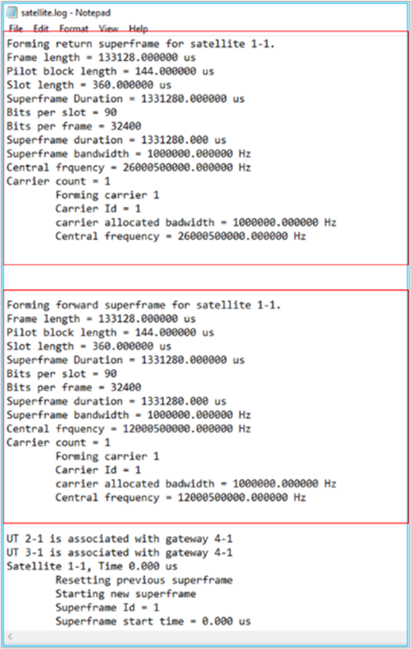
Figure-11: Satellite Radio Measurements log file
Omitted Features
Regenerative transponder where the signal is demodulated, decoded, re-encoded and modulated aboard the satellite.
Impact of Rain/Weather on signal propagation
Forward Error Coding in Layer 2
IPv6 Addressing
No support for LEO, MEO