Advanced Features
Random Number Generator and Seed Values
NetSim includes protocol and traffic models which include stochastic behavior. Typical examples are a) Wi-Fi node’s random back-off after collisions, and b) packet error decision by comparing a random number chosen between 0 and 1 against the packet error probability.
NetSim uses an in-built prime modulus combined with a linear congruential Random Number Generator (RNG) to generate the randomness. It is a single stream RNG with a period of \(\approx 2 \times 10^{18}\). Two seeds values are used to initialize the RNG. These seeds can be input from NetSim GUI or via the config file. Having the same set of seed values ensures that for a particular network configuration the same output results will be got, irrespective of the system or time at which the simulation is run. This ensures repeatability of experimentation.
Modifying the seed value will lead to the generation of a different stream of random numbers and thereby lead to a different sequence of events in NetSim. Therefore, all simulation results are dependent on the initial seeding of the RNG.
Confidence in simulation results and error bars
Since NetSim’s models include stochastic behavior, results are dependent on the initial seeding of the random number generator. Because a particular random seed selection can potentially result in an anomalous, or non-representative behavior, it is important for each model configuration to be exercised with several random number seeds, to be able to determine standard or typical behavior.
The field of statistics provides methods for calculating confidence in an estimate, based on a trial or series of random trials. To calculate confidence intervals, users can do the following:
Run \(N\) simulations for the same model configuration, with a different initial seed (for the random number generator) for each run.
For any output metric \(X\), calculate the mean (average) \(\overline{X}\) of the \(N\) samples.
\[\overline{X} = \frac{1}{N}\left( X_{1} + X_{2} + \ldots + X_{N} \right)\]
Calculate the standard deviation \(\sigma\) of the \(N\) samples.
\[\sigma = \sqrt{\left( \frac{1}{N - 1} \right) \times \Sigma\ \left( X_{i} - \overline{X} \right)^{2}}\]
Confidence interval limits can be expressed as
\[\Theta_{lower} = \overline{X} - z_{\alpha} \times \left( \frac{\sigma}{\sqrt{(N)}\ } \right),\ {\ \Theta}_{upper} = \overline{X} + z_{\alpha} \times \left( \frac{\sigma}{\sqrt{(N)}\ } \right)\]
This statement can be thought of as assigning a probability to the condition that the true mean \(\mu\) is within a particular distance of the random sample \(\overline{X}\), as shown below
\[Prob\ \left\lbrack \overline{X} - z_{\alpha} \times \left( \frac{\sigma}{\sqrt{(N)}\ } \right) < \mu < \ \overline{X} + z_{\alpha} \times \left( \frac{\sigma}{\sqrt{(N)}\ } \right) \right\rbrack = \alpha\]
| Confidence level (\(\mathbf{\alpha)}\) | \[\mathbf{z}_{\mathbf{\alpha}}\] |
|---|---|
| 99% | 2.575 |
| 98% | 2.327 |
| 95% | 1.960 |
| 90% | 1.645 |
| 80% | 1.282 |
Value of \(\mathbf{Z}_{\mathbf{\alpha}}\mathbf{\ }\) for different confidence intervals
The above expression for confidence assumes the distribution of the output metric is Normal, which is true (from the Central Limit Theorem) if the number of runs \(N \geq 30.\) If the number of repetitions is less than 30 then it is better to use the t-statistic based confidence-interval (details can be found in standard statistics textbooks).
Error bars are plotted as a vertical bar centered at the mean and ending at the upper and lower confidence limits
Interfacing MATLAB with NetSim (Std/Pro versions)
NetSim provides run-time interfacing with MATLAB so that users do not have to rewrite code in C for features that are already available in MATLAB and instead simply reuse MATLAB code. Lot of work related to machine learning, artificial intelligence and specialized mathematical algorithms which can be used for networking research, can be carried out using existing MATLAB code.

Interfacing MATLAB with NetSim
This interfacing feature can be used to either replace an existing functionality in NetSim or to incorporate additional functionalities supported by MATLAB. Any existing command /function/algorithm in MATLAB or a MATLAB M-script can be used.
In general, the following are done when a user interfaces NetSim to MATLAB:
Initialize a MATLAB engine process in parallel with NetSim,
Execute MATLAB workspace commands,
Pass parameters to MATLAB workspace,
Read parameters from MATLAB workspace,
Generate dynamic three-dimensional plots,
Make calls to functions that are part of MATLAB M-scripts or .m files, and
Terminate the MATLAB engine process at NetSim simulation end.
Guidelines to interface NetSim with MATLAB
Analyze what parameters the function or code in MATLAB expects as input.
Identify the relevant variables in NetSim to be passed as input to MATLAB.
Make calls from relevant places of NetSim source code to
Pass parameters from NetSim to MATLAB.
To read computed parameters from MATLAB workspace
Identify and update the appropriate simulation variables in NetSim.
NetSim offers Socket interfacing to interact with MATLAB during runtime.
The socket interface that offers simplified NetSim API’s that can be used for interactions with MATLAB. The steps are lot simpler since no additional settings will be required in the source code project settings.
NetSim-MATLAB Socket Interface
NetSim-MATLAB Socket Interface was introduced in NetSim v14.0. It provides several inbuilt APIs that can be called from the underlying protocol C source codes to interact with MATLAB. Following is some of the APIs with syntax and description:
| NetSim API’s to interact with MATLAB | Description |
|---|---|
| netsim_matlab_interface_configure(char* appPath) | Starts a MATLAB engine process and adds the appPath to the top of the search path for current MATLAB session. |
| netsim_matlab_interface_close(); | Sends exit command to MATLAB to terminate the session. |
| netsim_matlab_send_ascii_command(char* format, ...) | Sends commands, variables and values as string to MATLAB. |
| netsim_matlab_get_value(char* out, int outLen, char* name, char* type) | Gets the value of a MATLAB variable as a string. Currently supports double data type only. |
| ptrMXArray netsim_matlab_get_array(char* name) | This function retrieves a MATLAB matrix containing double-precision values specified by the variable name. It returns a pointer to an mxArray structure (ptrMXArray) with the following components: arr: A flat array containing all entries of the MATLAB matrix, irrespective of its dimensions. dimn: An array specifying the dimensions of the MATLAB matrix. shape: An array containing the size of each dimension. netsim_matlab_send_array |
| void netsim_matlab_send_array(double* arr, size_t* shape, size_t dimn, char* name) | This function sends a C array of double-precision values to MATLAB and creates an equivalent variable in MATLAB. It takes the following arguments: arr: The pointer to the C double type array. shape: An array representing the size of each dimension. dimn: The dimension of the array. name: The name of the equivalent MATLAB variable. |
MATLAB Engine API functions
These functions are defined as part of the NetSim_utility.h file which is part of the Include directory of NetSim Source Codes. This header can be included in the C files where these APIs are to be called from.
Prerequisites for MATLAB Socket Interfacing
An installed version of MATLAB R2023(b) or lower version in the same system where NetSim is installed.
Note: Execute the below command in the command prompt where MATLAB_Interface.exe is placed followed by IP address of the system where the NetSim is installed.

Command to start the MATLAB interface
Registration of MATLAB as a COM server by one of the following methods
Start Command Prompt as administrator and execute the following command:
matlab -regserver
Note: If you have multiple versions of MATLAB installed on your computer, the best practice is to run the matlab command from the matlab root folder.
Enter the following command in the command line of MATLAB version that you want to interface with NetSim:
matlab -regserver
Implement Weibull Distribution of MATLAB without using .m file
In this example we will replace the default Rayleigh Fading (part of the path loss calculation) used in NetSim, with a Fading Power calculated using the Weibull Distribution from MATLAB Socket Interfacing.
Procedure
Open NetSim Source codes in Visual Studio by going to Your Work -> Open, Reset and Compare option -> Open Code, in the Home Screen of NetSim.
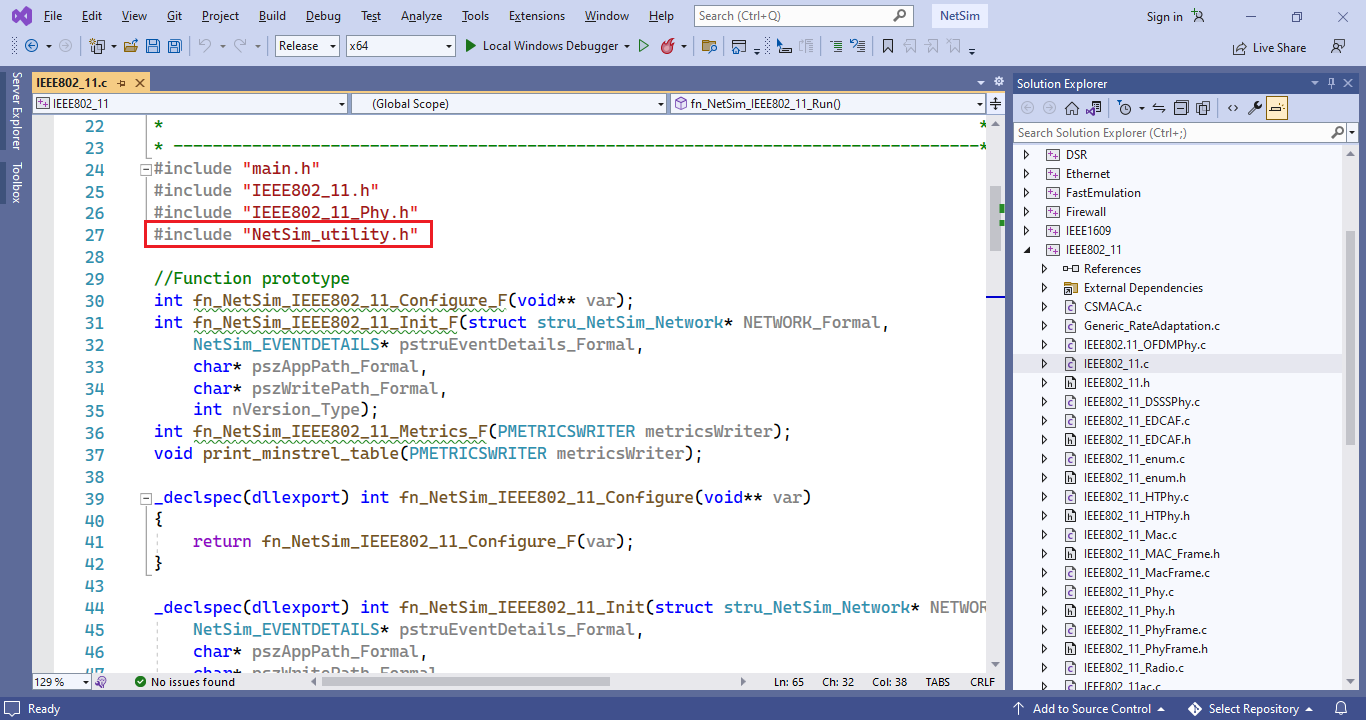
In the Solution Explorer under IEEE802_11 project double click on the IEEE802_11.c file.

Solution Explorer double click on the IEEE802_11.c file
The NetSim_utility.h header file is included in IEEE802_11.c
 Figure
10‑4: NetSim_utility.h file in IEEE802_11.c file
Figure
10‑4: NetSim_utility.h file in IEEE802_11.c file
Add a call to netsim_matlab_interface_configure() API, passing pszAppPath as an argument, inside the fn_NetSim_IEEE802_11_Init() function.

Adding a call to netsim_matlab_interface_configure API inside the fn_NetSim_IEEE802_11_Init() function
Similarly add a call to netsim_matlab_interface_close(); inside the fn_NetSim_IEEE802_11_
Finish() function.

Adding a call to netsim_matlab_interface_close() API inside the fn_NetSim_IEEE802_11_Finish() function
In the Solution Explorer under expand the Medium project and double click on the Medium.c file.
Add a line in the beginning of the file to include the NetSim_utility.h header file.
 Figure 10‑7: Including the
NetSim_utility.h file in Medium.c file
Figure 10‑7: Including the
NetSim_utility.h file in Medium.c file
Define a new function static double matlab_calculate_fadingloss() above the existing static void medium_mark_packet_error(ptrPACKETINFO info) function.
static double matlab_calculate_fadingloss()
{
char buf[BUFSIZ];
double result;
int weibull_noncentrality = 1, weibull_scale = 2;
//use ProbDistUnivParam() function for matlab 2016 or lower
//sprintf_s(buf, BUFSIZ, "h=ProbDistUnivParam('weibull',[%d %d])",
//weibull_noncentrality, weibull_scale);//
//use makedist() function for matlab 2017 or Higher
sprintf_s(buf, BUFSIZ, "h=makedist('weibull',%d,%d)", weibull_noncentrality,
weibull_scale);
netsim_matlab_send_ascii_command(buf);
sprintf_s(buf, BUFSIZ, "i=random(h)");//
netsim_matlab_send_ascii_command(buf);
netsim_matlab_get_value(buf, BUFSIZ, "i", "double");
result = atof(buf);
return result;
}
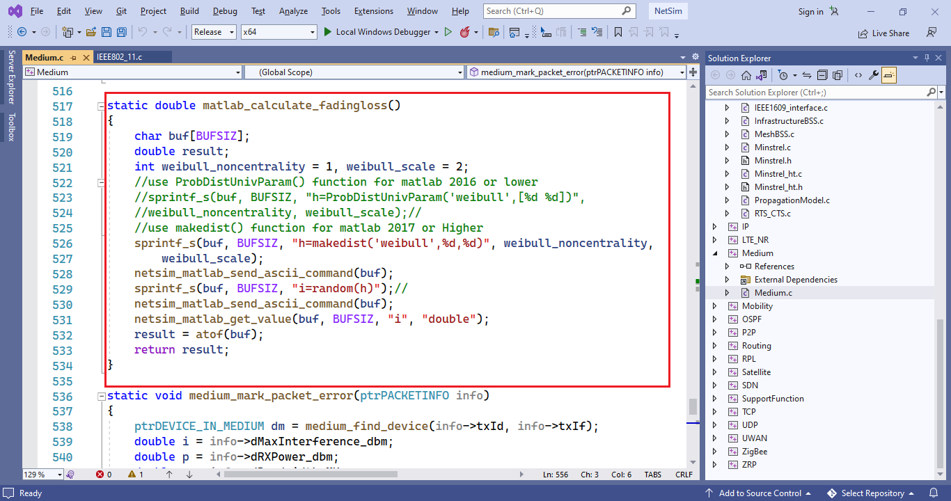 Figure 10‑8: Defining a new
function matlab_calculate_facingloss() in the Medium.c file
Figure 10‑8: Defining a new
function matlab_calculate_facingloss() in the Medium.c file
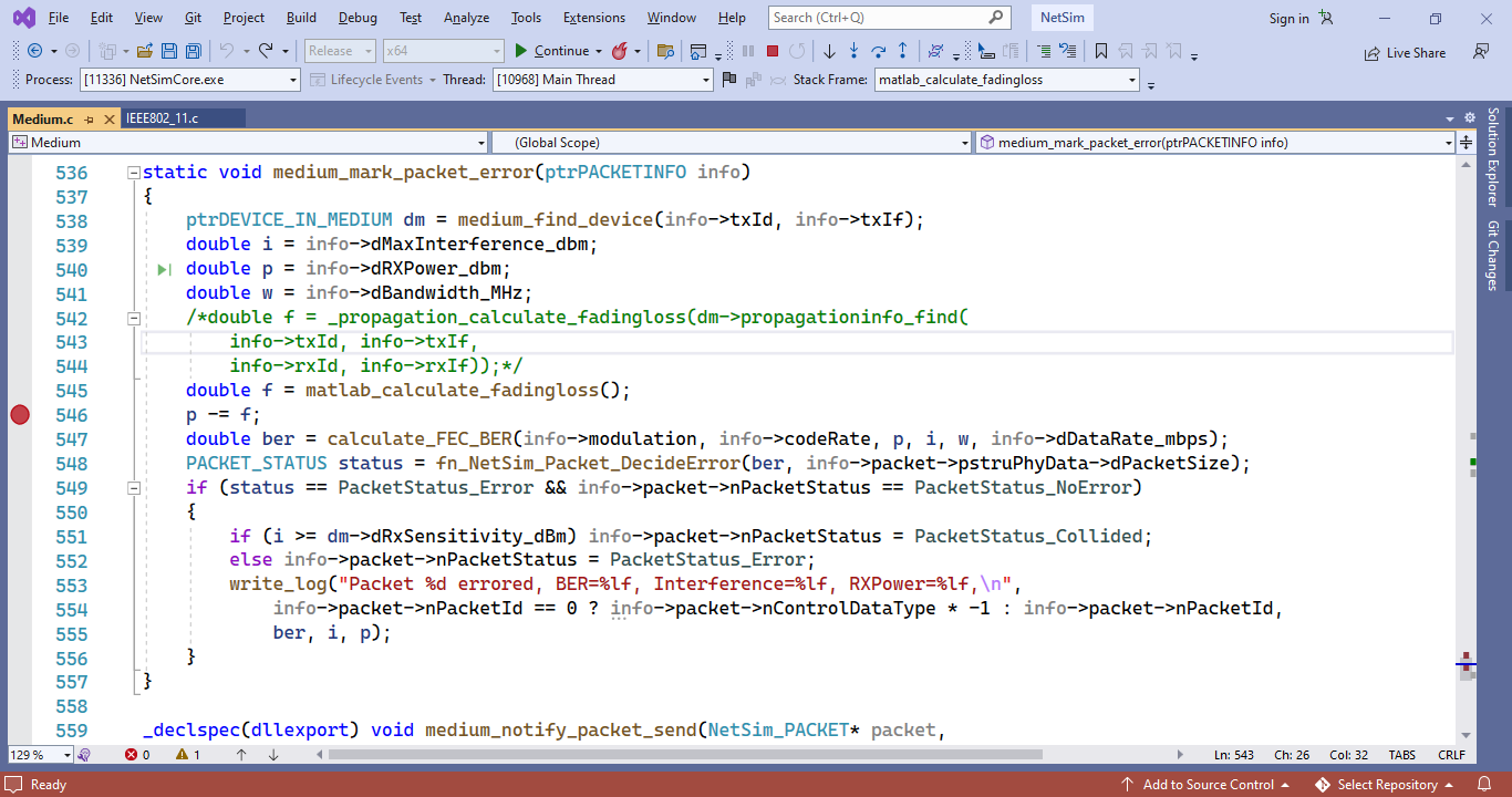
Inside medium_mark_packet_error() function comment the lines,
double f = _propagation_calculate_fadingloss(dm->propagationinfo_find(
info->txId, info->txIf,
info->rxId, info->rxIf));
Make a call to the fn_netsim_matlab_run() function by adding the following line,
double f = matlab_calculate_fadingloss();

Call to the matlab_caculate_fadingloss() function
Note: In MATLAB Socket Interfacing, compilation of MATLAB Engine is not required since the MATLAB APIs are already called in function.
Now rebuild the IEEE802_11 and Medium source code projects one after the other, by right clicking on the project and selecting Rebuild option.
Upon successful build, NetSim automatically takes care of updating the binaries of IEEE802_11 and Medium source code projects which will be used for further simulations.
Run NetSim in Administrative mode. Create a Network scenario involving IEEE802_11 say MANET, right click on the Adhoc link and select properties. Make sure that the Channel Characteristics is set to PathLoss and Fading and Shadowing. Perform the simulation.

Wireless Link Properties Window in MANET
If MATLAB is installed in the same system where NetSim is installed. MATLAB Interface process can be initiated directly from the design window of NetSim.
Go to “Options” in design window and select the Open MATLAB Interface option as shown below:
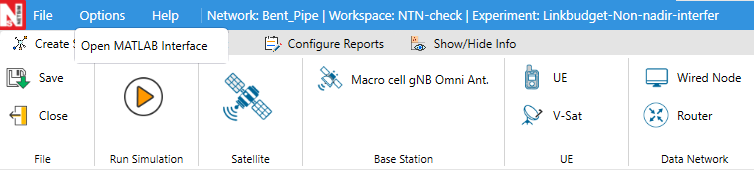
Option to open MATLAB Interface
Click on the OK when the below window is displayed. This opens the MATLAB Session.

NetSim MATLAB Interfacing warning message
After clicking on “OK”, MATLAB interface will get initiated. MATLAB Command window will open as shown below
Click on run simulation ,after which the simulation NetSim starts to simulate. During the simulation communication between MATLAB and NetSim will be established as shown below
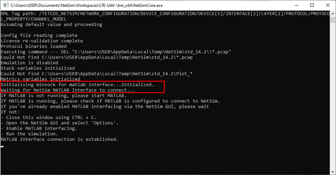

NetSim Simulation console for MATLAB Interface process to connect
The dFading power value will be displayed in the MATLAB Console window as below. At simulation end the MATLAB Interface process will get terminated.

Runtime MATLAB interfacing window with I value
Debug and understand communication between NetSim and MATLAB
In the Solution Explorer under Medium project double click on Medium.c file and place a breakpoint inside the matlab_calculate_fadingloss() function before the return statement.

Placing a breakpoint inside matlab_calculate_fadingloss() function
Now run the NetSim Scenario. The simulation window stops for user interrupt.
In Visual studio, go to Debug =>Attach to Process.
From the list of Processes select NetSimCore.exe and click on Attach.

Select NetSimCore.exe in Attach to Process Window
Now go to the Simulation window and press Enter. Simulation will pause at Waiting for matlab interface to connect, go to Design window/GUI -> Options -> Open MATLAB interface ->click on OK
MATLAB Command Window will start and breakpoint in Visual Studio gets triggered.

Breakpoint getting triggered in Visual Studio.
Now place another breakpoint after the line double f = matlab_calculate_fadingloss(); in the function medium_mark_packet_error() function and press continue or F5 key.
Adding Breakpoint under in the medium_mark_packet_error() function
Once the second breakpoint gets triggered, add the variable f which stores the fadingloss value, in Medium.c file, to watch. For this, right click on the variable f and select “Add Watch” option. You will find a watch window containing the variable name and its value in the bottom left corner.

Right Clicking on the variable f and adding it to Watch
Now when debugging (say by pressing F5 each time) you will find that the watch window displays the value of f whenever the control reaches the recently set breakpoint. You will also find that the value of f shown in the Visual Studio Watch window and the value of i in the MATLAB Console window are similar.

The Visual Studio Watch window variable f and the value of i in the MATLABInterface window are similar
Implement Weibull Distribution of MATLAB in NetSim using .m file
Procedure:
Create a file weibull_distribution.m file with the following code:
function out= weibull_distribution(noncentrality,scale)
%use ProbDistUnivParam() function for matlab 2016
%h=ProbDistUnivParam('weibull',[noncentrality,scale]);
%use makedist() function for matlab 2017
h=makedist('weibull',noncentrality,scale);
i=random(h,1);
out=i;
end
Create matlab folder inside the bin_x64 directory of the current workspace
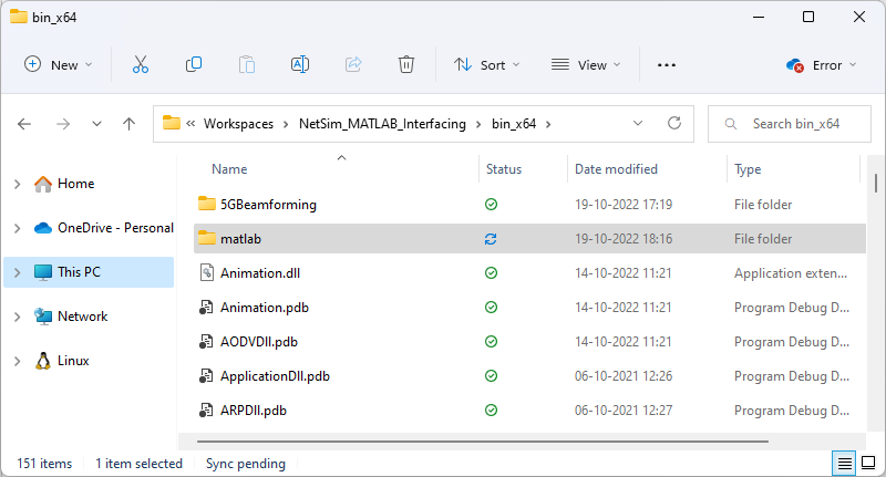
Bin folder of x64 of current workspace
Place the weibull_distribution.m file inside matlab folder.

Place Weibull_distribution.m file inside matlab folder
Modify the function static double matlab_calculate_fadingloss() that we previously created in the Medium.c file to call the newly created Weibull_distribution.m
static double matlab_calculate_fadingloss()
{
char buf[BUFSIZ];
double result;
int weibull_noncentrality = 1, weibull_scale = 2;
//use ProbDistUnivParam() function for matlab 2016 or lower
//sprintf_s(buf, BUFSIZ, "h=ProbDistUnivParam('weibull',[%d %d])",
//weibull_noncentrality, weibull_scale);//
//use makedist() function for matlab 2017 or Higher
sprintf_s(buf, BUFSIZ, "k=weibull_distribution(%d,%d)", weibull_noncentrality,
weibull_scale);
netsim_matlab_send_ascii_command(buf);
netsim_matlab_get_value(buf, BUFSIZ, "k", "double");
netsim_matlab_send_ascii_command(buf);
result = atof(buf);
return result;
}
Right click on the Medium source code project and select Rebuild.
Proceed to run simulation as explained in the previous sections.
You will find that once the Simulation is run MATLAB Command Window starts to execute and fadngloss value will be printed based on the call to weibull_distribution.m file.

Runtime MATLAB interfacing window with k value
Interfacing Python with NetSim
NetSim provides run-time interfacing with Python so that users do not need to rewrite code in C for functionalities that already exist in Python. Instead, users can reuse existing Python libraries. A large amount of work related to machine learning, artificial intelligence, data analytics, and mathematical modeling—which can be valuable for networking research—can be directly implemented using existing Python packages such as NumPy, SciPy, TensorFlow, scikit-learn, etc.

Interfacing Python with NetSim
This interfacing feature can be used to either replace existing functionalities in NetSim or add new features that are better supported in Python. Any existing Python script, module, or function can be invoked from within the NetSim simulation environment.
In general, the following are done when a user interfaces NetSim to Python:
Initialize a Python script or server process that communicates with NetSim.
Send parameters from NetSim to Python.
Receive results or computed outputs from Python.
Handle various data types via structured message formats.
Make calls to user-defined Python functions or modules.
Guidelines for Interfacing NetSim with Python
Determine which parameters, variables or results from NetSim need to be passed to Python.
Run the Python script that listens for NetSim connections.
Use the provided NetSim socket API functions to package and send data.
Make calls from relevant places of NetSim source code to
Pass parameters from NetSim to Python.
Data are serialized into byte streams, transferred via sockets, and deserialized in Python.
The Python side automatically reconstructs received segments into native types.
Users can directly operate on them, perform computations, and send results back.
Identify and update the appropriate simulation variables in NetSim.
NetSim offers Socket interfacing to interact with Python during runtime.
This socket interface exposes simplified NetSim APIs for bidirectional communication with Python, making the integration process easier. Since socket-based communication does not require additional compiler or project settings, users can quickly connect NetSim simulations with external Python scripts for dynamic computation, visualization, or automation.
NetSim-Python Socket Interface
It provides several inbuilt APIs that can be called from the underlying protocol C source codes to interact with Python. Following are some of the APIs with syntax and description:
| NetSim API’s to interact with Python | Description |
|---|---|
| void* Init_netsim_python_Interface() | Initializes a socket and waits for a connection from python. This must be called once before any data exchange begins. |
| Message* Init_Message() | Allocates and initializes a new message structure used to send data segments from NetSim to Python. Call this before adding variables you want to send to Python. |
| void add_variable_to_message(void* message_v,….,VAR_END) | Adds one or more variables (int, double, string, arrays, etc.) into a message. |
| SEGMENT* msg_get_value(MESSAGE* m); void msg_reset(MESSAGE* m) |
msg_get_value() helps retrieves the next
segment in the message based on internal cursor. msg_reset() will reset the message internal cursor so you can read variables again from the beginning. |
| int send_receive_message(void* handle, void* message_v, void** outMessage) | Sends a message containing simulation data to Python, and receives the reply if Python sends any data. |
| uint32_t get_variablecount(void* message_v) | Returns the total number of variables (segments) currently present in the given message. |
| void debug_print_message(MESSAGE* m, int want_raw) | Prints the contents of a message (both variable names and values) to the console or log file. |
| void free_message(void* message_v) | Frees all dynamically allocated memory associated with a message, including its segments and data buffers. Must be called once a message is no longer needed to prevent memory leaks. |
| int init_logging(const char* path, int to_console) | Initializes the logging system, used to
log all internal operations in a file. Can change the settings to log anything on display(terminal). |
| void netsim_python_interface_start(char* filepath) | Starts the Python Client program automatically, without having to start it manually. The path to the file, including the filename has to be passed as an argument. |
LOG_INFO() LOG_ERR() |
These functions help with logging, which is initiated by init_logging. |
Interface API functions (NetSim Side)
These functions are defined as part of the
NetSim_Python_Interface.h file which is part of the Include
directory of NetSim Source Codes. This header can be included in the C
files where these APIs would be used. To know more details about how to
use the functions, see the header file
(NetSim_Python_Interface.h).
Similarly, APIs on the python side are defined. Following is some of the
APIs with syntax and description:
| Python API’s to interact with Netsim | Description |
|---|---|
| connect(host,port) | Establishes a TCP connection to NetSim. Must be called before sending or receiving any messages. |
| Message() | Creates a new empty message object. Each message can contain multiple variables of different data types. |
| add_variable(message, var_type, value, length) | Adds a variable or array (int, double, bool, string, etc.) into a Message. Call this once per value or array you want to send. |
| get_value() and reset_cursor() | get_value() retrieves variables from a
received message one segment at a time. reset_cursor() moves the message
cursor back to the beginning so values can be read again. These are methods defined under Message class. |
| send_and_receive(socket, message, expect_reply) | Send a prepared message to NetSim and optionally receivethe reply message. |
| debug_print_message(message, want_raw, title) | Prints all variables inside a message for debugging. can also display raw bytes if required. |
| setup_logging(log_path, to_console, to_file) | Enables logging for all Python–NetSim communication. Logs can be written to console or file for debugging and troubleshooting. |
Interface API functions (Python Side)
These functions are defined as part of the netsim_socket_client.pyd file that can be found inside NetSim_Python_Interface_Client directory of NetSim Simulation source code folder. This will be required to call above functions. Add your Python code to the directory NetSim_Python_Interface_Client and import the functions that you want to call.
To know more details about how to use the functions see the sample python file (sample.py) that is available in the NetSim_Python_Interface_Client directory.
Prerequisites for Python Socket Interfacing
Before using the NetSim–Python interface, ensure that your Python environment is properly configured and compatible with NetSim’s socket communication layer.
Python 3.8 or higher (recommended: 3.10+). Earlier versions are not supported due to differences in socket and multiprocessing behavior.
The following standard or third-party modules are required:
Socket, Struct, logging, numpy
Ensure that the chosen socket port (5555) is not blocked by a firewall or already in use.
Interfacing tail with NetSim
What is a tail command?
The tail command is a command-line utility for outputting the last part of files given to it via standard input. It writes results to standard output. By default, tail returns the last ten lines of each file that it is given. It may also be used to follow a file in real-time and watch as new lines are written to it.
PART 1:
Tail options
The following command is used to log the file.
tail " path_to_file " -f
where -f option is used to watch a file for changes with the tail command pass the -f option. This will show the last ten lines of a file and will update when new lines are added. This is commonly used to watch log files in real-time. As new lines are written to the log the console will update will new lines.
If users do not want the last ten lines of the file, then use the following command.
tail -n 0 " path_to_file " –f
where –n option is used to show the last n number of lines.
If you want to open more than 1 file then use the following command
tail –n 0 " path_to_file " " path_to_file " –f
PART 2:
Steps to log NetSim files using tail console.
Note: Before Executing below steps, User need to generate/Simulate a scenario of a network with specific network logs enabled to which tail command is being executed.
Open command window from Install directory path of Netsim (<C:\Program Files\NetSim\Pro_v14_4\bin) which contains tail.exe
Type the following command to open ospf_hello.log.txt file and press enter.
tail -n 0 “<NetSim_IOPath>\log\ospf_hello.log” -f
For example,
tail -n 0 "C:\Users\ALICE\AppData\Local\Temp\NetSim\pro_14.4\log\log\ospf_hello.log" -f

Enter the ospf_hello.log.txt file path is Command Prompt
Open solution file and add the following line in fn_NetSim_OSPF_Init() function in ospf.c file present inside OSPF project

Add the following line in fn_NetSim_OSPF_Init() function in ospf.c file present inside OSPF project
Rebuild the project.
Upon rebuilding, libOSPF.dll will get created in the bin folder of NetSim’s current workspace path <C:\Users\PC\Documents\NetSim\Workspaces\<Your default workspace>\bin_x64 > for 64-bit
Create a scenario in NetSim as per the screenshot below and run simulation.

Network Topology
In the console window user would get a warning message shown in the below screenshot Figure 10‑27 (because of changed DLL) and then the simulation will pause for user input (because of _getch() added in the init function)

Modified Project DLL Warning Message in NetSim Console
In Visual Studio, put break point inside all the functions in OSPF_Hello.c file present inside OSPF project.
Go to “Debug->Attach to Process” in Visual studio and attach to NetSimCore.exe.
Press enter in the command window. Then control goes to the project and stops at the break point in the source code as shown below Figure 10‑28.

Control goes to the project and stops at the break point in the source code.
Once after pressing enter in command window, check the tail console to watch the ospf_hello.log would look like the following screenshot Figure 10‑29.
Below Screenshot shows that scheduling time of hello interval for each Routers connected in Network.

Scheduling hello interval for Routers.
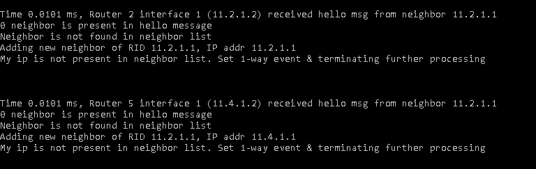
Adding new neighbor and terminating process if it is 1-way event
Above Screenshot shows of adding neighbor to hello message, at Time 0.0101 ms, Router 5 interface 1 (11.4.1.2) received hello msg from neighbor 11.2.1.1.
Adding Neighbor and Performing 2-way Event if neighbor is present in Router’s list.
Above Screenshot indicates the Router 2’s interface 1 (11.2.1.2) has received hello message from neighbor 11.2.1.1, if neighbor is present in Router’s list 2-way event will be performed.
Similarly, users can debug the code and observe how the OSPF tables get filled.
Users can also open multiple files by using the command given in Part 1.
Adding Custom Performance Metrics
NetSim allows users to add additional metrics tables to the Simulation Results window in addition to the default set of tables that are available at the end of any simulation. This can be achieved by editing the source codes of the respective protocol.
General format to add custom metrics in Result window:
Every protocol has a main C file which contains a Metrics () function. For E.g., TCP project will have a TCP.c file, UDP will have an UDP.c file etc. In the following example we have added a new table as part of TCP protocol. TCP.c file contains fn_NetSim_TCP_Metrics() function where code related to custom metrics is added as shown below:
_declspec(dllexport) int fn_NetSim_TCP_Metrics(PMETRICSWRITER metricsWriter)
{
//CUSTOM METRICS
//Set table name
PMETRICSNODE table = init_metrics_node(MetricsNode_Table, "CUSTOM METRICS", NULL);
//set table headers
add_table_heading(table, "COLUMN_HEADER_1", true, 0);
add_table_heading(table, "COLUMN_HEADER_2", false, 0);
//Add table data
add_table_row_formatted(false, table, "%s,%s,", "ROW_DATA1","ROW_DATA2");
PMETRICSNODE menu = init_metrics_node(MetricsNode_Menu,"CUSTOM_METRICS", NULL);
//Add table to menu
add_node_to_menu(menu, table);
//Write to Metrics file
write_metrics_node(metricsWriter, WriterPosition_Current, NULL, menu);
delete_metrics_node(menu);
//CUSTOM METRICS
return fn_NetSim_TCP_Metrics_F(metricsWriter);
}

Added Custom metrics table to the Additional metrics window.
For illustration, an example regarding Wireless Sensor Network is provided. In this example, parameters such as Sensor Node Name, Residual Energy, State (On/Off) and turn–off time are tracked and added to a new table in the Simulation Results window.
Refer Section 9.1 on writing your own code, for more information.
After loading the source codes in Visual Studio, perform the following modifications:
Step 1: Copy the provided code at the top in 802_15_4.h file present in Zigbee project.
double NetSim_Off_Time[100]; //Supports upto Device ID 100. Array size can be increased for higher number of Devices/Device ID's
Step 2:
Add the header file in 802_15_4.c file.
#include "../BatteryModel/BatteryModel.h"
Step 3:
Copy the below code (in red colour) in 802_15_4.c file (inside fn_NetSim_Zigbee_Metrics() function)
/** This function write the metrics in metrics.txt */
_declspec(dllexport) int fn_NetSim_Zigbee_Metrics(PMETRICSWRITERmetricsWriter)
{
//CUSTOM METRICS
ptrIEEE802_15_4_PHY_VAR phy;
ptrBATTERY battery;
char radiostate[BUFSIZ];
NETSIM_ID nDeviceCount = NETWORK->nDeviceCount;
//Set table name
PMETRICSNODE table = init_metrics_node(MetricsNode_Table, "NODE_FAILURE_METRICS", NULL);
//set table headers
add_table_heading(table, "Node Name", true, 0);
add_table_heading(table, "Status(ON/OFF)", true, 0);
add_table_heading(table, "Residual_Energy (mJ)", true, 0);
add_table_heading(table, "Time - Turned OFF (microseconds)", false, 0);
for (int i = 1; i <= nDeviceCount; i++)
{
sprintf(radiostate, "ON");
phy = WSN_PHY(i);
if (strcmp(DEVICE(i)->type, "SENSOR"))
continue;
if (WSN_MAC(i)->nNodeStatus == 5 || phy->nRadioState==RX_OFF)
sprintf(radiostate, "OFF");
//Add table data
if(phy->battery)
add_table_row_formatted(false, table, "%s,%s,%.2lf,%.2lf,", DEVICE_NAME(i), radiostate, battery_get_remaining_energy((ptrBATTERY)phy->battery), NetSim_Off_Time[i]);
}
PMETRICSNODE menu = init_metrics_node(MetricsNode_Menu, "CUSTOM_METRICS", NULL);
add_node_to_menu(menu, table);
write_metrics_node(metricsWriter, WriterPosition_Current, NULL, menu);
delete_metrics_node(menu);
//CUSTOM METRICS
return fn_NetSim_Zigbee_Metrics_F(metricsWriter);
}
Step 4:
Copy the below code (in red colour) at the end of ChangeRadioState.c file.
if(isChange)
{
phy->nOldState = nOldState;
phy->nRadioState = nNewState;
}
else
{
phy->nRadioState = RX_OFF;
WSN_MAC(nDeviceId)->nNodeStatus = OFF;
NetSim_Off_Time[nDeviceId] = ldEventTime;
}
return isChange;
}
Step 5:
Build DLL with the modified code and run a Wireless Sensor Network scenario by considering power source as battery model. After Simulation, user will notice a new Performance metrics named “Custom Metrics” is added. The newly added NODE_FAILURE_METRICS table is shown below Figure 10‑33.

Added Custom metrics table to the Additional metrics window.
Simulation Time and its relation to Real Time (Wall clock)
The notion of time in a simulation is not directly related to the actual time that it takes to run a simulation (as measured by a wall-clock or the computer's own clock), but is a variable maintained by the simulation program. NetSim uses a virtual clock which ticks virtual time. Virtual time starts from zero progresses as a positive real number.
Time is as a global parameter. All components of the network share the same time throughout the simulation independently of where they are physically located or how they are logically connected to the network. There are not differences among the local time of the communication network components.
This virtual time is referred to as simulation time to clearly distinguish it from real (wall-clock) time. NetSim is a discrete event simulator (DES), and in any DES, the progression of the model over simulation time is decomposed into individual events where change can take place. The flow of time is only between events and is not continuous. Therefore, simulation time is not allowed to progress during an event, but only between events. In fact, the simulation time is always equal to the time at which the current event occurs. Thus, simulation time can be viewed as a variable that "jumps" to track the time specified for each new event.
The answer to the question "Will NetSim run for 10 seconds if Simulation time is set to 10 sec?" is, the simulation may take more than 10 seconds (Wall clock) if the network scenario is very large and heavy traffic load. It may take a much shorter time (wall clock) for small networks with low traffic loads.
Note that when running in "Emulation mode" simulation time and wall clock will be exactly synchronized since it involves the transfer of real packets across the virtual network in NetSim.
In NetSim, the current simulation time can be got using -pstruEventDetails->dEventTime
Environment Variables in NetSim
NETSIM_PACKET_FILTER = <filter_string> //used by NetSim developers to debug. Emulator code to passes filter string to windivert. See windivert doc for more information.
NETSIM_EMULATOR_LOG = <log_file_path> // Used by Real time sync function to log get event and add event. Used by NetSim developers to debug.
NETSIM_EMULATOR = 1 // Set by application DLL or user to notify NetSim internal modules to run in emulation mode
NETSIM_CUSTOM_EMULATOR = 1 // To notify NetworkStack to not load emulation DLL and to only do time sync.
NETSIM_SIM_AREA_X = <int> // Area used by Mobility functions for movement of device. Set by config file parser or user.
NETSIM_SIM_AREA_Y = <int> // Same as above
NETSIM_ERROR_MODE = 1 // if set then windows won't popup gui screen for error reporting on exception.
NETSIM_BREAK = <int> // Event id at which simulation will break and wait for user input.
Equivalent to -d command in CLI mode.
NETSIM_IO_PATH = <path> // IO path of NetSim from where it will read Config file and write output file. Equivalent to -IOPATH command in CLI mode.
NETSIM_MAP = 1 // Set by Networkstack to inform other modules that simulation is running per map view.
NETSIM_ADVANCE_METRIC // If set, NetSim provides a set of extra metrics.
In application metrics, you can see duplicate packets received.
NETSIM_CONFIG_NAME = <FILE NAME> // Config file name. This file must present in IOPath. If not set default value is Configuration.netsim
NETSIM_NEG_ID = 1 // If set, then control packets will have negative id.
NETSIM_PACKET_DBG = 1 // If set, then Simulation engine will log the packet creation and freeing
NETSIM_MEMCHECK = 1 // If set, then simulation will enable memory check.
NETSIM_MEMCHECK_1 = x // Lower event id
NETSIM_MEMCHECK_2 = x // Upper event id
Best practices for running large scale simulations
As we scale simulations, the number of events processed and the memory consumed increase. Simulation scale can be defined in terms of:
Number of Nodes
End nodes
Intermediate devices
Total traffic in the network
Number of traffic sources
Average generation rate per source
Simulation time
The simulators performance is additionally affected by:
Protocols running
Network Parameters such as Topology, Mobility, Wireless Channel etc.
Enabling/Disabling - Plots, Traces and Logs
External Interfacing – MATLAB, Wireshark, SUMO
NetSim GUI limitation on total number of Nodes is as follows:
NetSim Academic:
Intermediate devices: 20
End nodes: 100
NetSim Standard:
Intermediate devices: 100
End nodes: 500
NetSim Professional :
Intermediate devices: 500
End nodes: 2500
Recommended best practices for running large scale simulations are:
Run 64-bit Build of NetSim
Use the latest Windows 10 Build.
Use a system running a high-end processor with minimum 32 GB RAM
Disable plots, traces and logs to speed up the simulation.
NetSim writes one packet trace and one event trace file per simulation. If users wish to open this file in MS-Excel, please note Excel’s limit of 1 Million rows.
Packet trace and Event trace can be disabled to speed up the simulation.
Running simulations via CLI mode will save memory.
Batch experimentation and automated simulations
NetSim Batch Automation allows users to execute a series of simulations without manual intervention. Consider a requirement, where a user wishes to create and simulate hundreds of network scenarios and store and analyse the performance metrics of each simulation run. It is impossible to do this manually using the GUI. This requirement can be met using NetSim Batch Automation script which runs NetSim via CLI.
A related requirement of advanced simulation users is a multi-parameter sweep. When you sweep one or more parameters, you change their values between simulation runs, and compare and analyze the performance metrics from each run.
The documentation and codes for batch experimentation script is available TETCOS - https://www.tetcos.com/file-exchange.html